
Flow Matching#
Flow matching is a deterministic transport method for generative modeling. It starts from a simple source distribution and learns a velocity field that carries samples toward the data distribution.
The probability-flow ODE already showed that a diffusion model can generate by integrating a deterministic field: once the score is known, sampling reduces to solving an ODE from noise to data. Flow matching takes that deterministic, ODE-based view as its starting point. It prescribes a probability path from the source to the data directly and learns the transport velocity along that path by regression, so the velocity field becomes the primary trained object instead of a quantity recovered from a noising process.
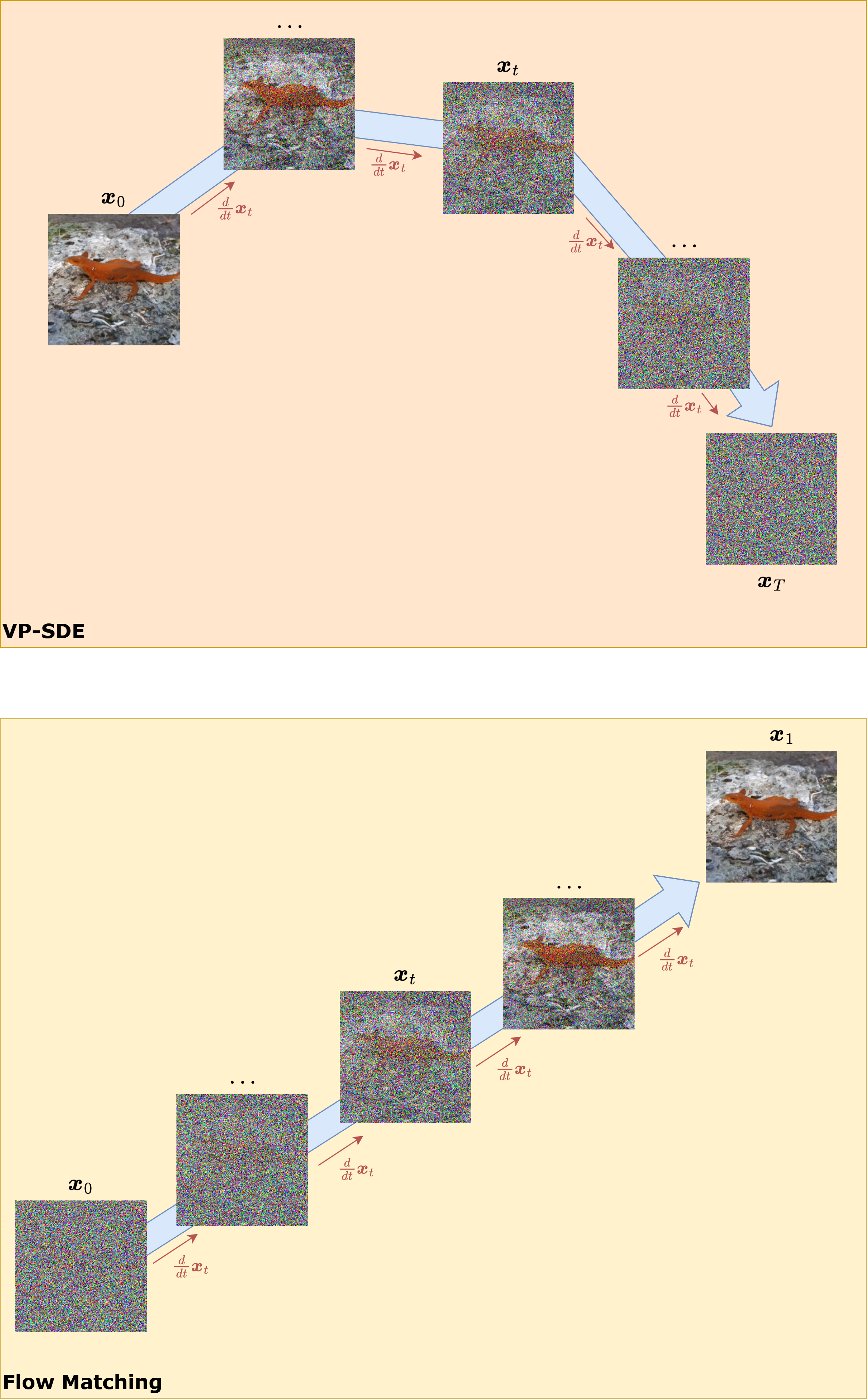
Fig. 46 Flow matching next to the variance-preserving diffusion path. Both connect a simple source distribution to the data distribution through a family of intermediate distributions. The VP-SDE reaches its generative field through a fixed noising process and the score that must be learned along it, while flow matching prescribes the path from source to data and learns the transport velocity along it directly.#
Deterministic transport and probability paths provide the foundation, conditional paths make the training target tractable, and a rectified-flow model on FashionMNIST turns the construction into a working image generator, in the same image setting used throughout the earlier chapters.
Important
Flow matching separates path design from field learning. The path specifies how source samples are connected to data samples. The neural network learns the velocity field associated with that path.
Deterministic Transport and Probability Paths#
The mental image behind flow matching is simple. Picture the source distribution as a large cloud of points scattered according to \(p_0\), for example a cloud of Gaussian noise samples. Generating data means moving every point in that cloud until the cloud as a whole takes the shape of the data distribution. Nothing is created or destroyed along the way; the points are only transported from where they start to where they should end up.
To move the points, we attach to every location and every instant a small arrow telling a point which direction to go and how fast. This collection of arrows is a velocity field, written \(\boldsymbol{v}(\boldsymbol{x}, t)\). A single point follows the field by obeying the ordinary differential equation
which just says: at time \(t\), while sitting at position \(\boldsymbol{x}(t)\), move in the direction \(\boldsymbol{v}\). Starting from a random point \(\boldsymbol{x}(0) \sim p_0\) and following the arrows until \(t = 1\) produces one generated sample. Doing this for the whole cloud transports the entire distribution.
A familiar version of the same picture is a drop of colored dye carried by flowing water. The amount of dye at a fixed spot rises or falls only because the water carries dye into or out of that spot. Probability density behaves the same way: as the points flow, the density at each location changes according to how much probability mass the velocity field is pushing in or out. Flow matching is the search for the velocity field whose flow gradually reshapes the source cloud \(p_0\) into the data distribution \(p_{\mathrm{data}}\).
This conservation-of-mass idea has an exact mathematical form, the continuity equation:
Each term has a plain reading. The first term, \(\partial_t p_t(\boldsymbol{x})\), measures how fast the density is changing in time at a point. The second term measures the net flow of probability into or out of that point produced by the velocity field. Requiring their sum to be zero is exactly the statement that probability is neither created nor destroyed, only carried around by the flow. This is the only fact about the flow that the rest of the chapter relies on: the velocity field and the evolving density are tied together by this balance.
For readers who want the precise statement, the balance law can be written down and proved in a few lines using integration by parts.
Theorem 20 (Continuity equation for deterministic flows)
Suppose \(\boldsymbol{x}(t)\) solves
and let \(p_t\) denote the density of \(\boldsymbol{x}(t)\). Under standard regularity assumptions,
Proof. Let \(\varphi\) be a smooth compactly supported test function. By the chain rule,
Writing the expectation against the density \(p_t\) gives
Integrating by parts moves the gradient onto the flux term and yields
Since this holds for every test function \(\varphi\), the bracketed quantity must vanish.
The next ingredient is a probability path \((p_t)_{t \in [0,1]}\) with \(p_0\) easy to sample and \(p_1 = p_{\mathrm{data}}\). In practice, \(p_0\) is often a standard Gaussian and \(p_{\mathrm{data}}\) is the data distribution. Once the path is chosen, the modeling problem becomes learning a vector field whose induced flow pushes \(p_0\) through the intermediate marginals and reaches \(p_{\mathrm{data}}\) at time one.
The important conceptual separation is this: in flow matching, path design and field learning are different decisions. The path is a modeling choice. The vector field is the trainable object.
Diffusion begins from a known corruption process and learns how to reverse it. Flow matching defines a connection between source samples and data samples directly, then learns the velocity consistent with that connection. Both are path-based generative models, and the deterministic core is the same one met through the probability-flow ODE. What differs is the predicted object: diffusion predicts noise or score-related quantities, while flow matching predicts transport velocities.
Let \(\boldsymbol{x}_0 \sim p_0\) and \(\boldsymbol{x}_1 \sim p_{\mathrm{data}}\). A simple conditional path is the linear interpolation
Conditionally on the endpoints, its instantaneous velocity is
This is already enough to generate a useful supervised target for learning.
Numerical Example: A Straight Conditional Path
Let \(\boldsymbol{x}_0 = (0,0)\) and \(\boldsymbol{x}_1 = (4,2)\). Then the linear path is \(\boldsymbol{x}_t = (4t, 2t)\). At time \(t = 0.25\), the intermediate point is \((1, 0.5)\) and the conditional velocity is still \((4,2)\). In other words, the local instruction given to the model is: “if you are at \((1,0.5)\) at time \(0.25\) for this endpoint pair, keep moving in the direction \((4,2)\).”
One such instruction is trivial. The power of flow matching comes from averaging many such local instructions across many endpoint pairs until a coherent global transport field emerges.
A single pair of endpoints defines a single path. The learned vector field must combine many such local instructions across overlapping regions of space and time. The model learns a global transport law from many endpoint pairs.
Theorem 21 (Conditional flow matching target)
Let \((\boldsymbol{x}_0, \boldsymbol{x}_1)\) be sampled from a coupling of \(p_0\) and \(p_{\mathrm{data}}\). Let \(\boldsymbol{x}_t\) be sampled from a conditional interpolation law \(p_t(\boldsymbol{x} | \boldsymbol{x}_0, \boldsymbol{x}_1)\) with conditional velocity target \(\boldsymbol{u}_t(\boldsymbol{x} | \boldsymbol{x}_0, \boldsymbol{x}_1)\). Then the minimizer of
is
Proof. For fixed \((\boldsymbol{x}, t)\), the loss is a squared-error regression problem whose random target is the conditional velocity. The minimizer of squared error is the conditional expectation of that target given the input. Applying that fact pointwise yields the claim.
This theorem contains the practical heart of the method. Once the conditional path is chosen, generative learning becomes squared-error regression on velocity targets. Diffusion has a similar supervised-learning structure, with denoising targets in place of transport velocities.
Flow Matching as Velocity Regression#
Continuous normalizing flows also use an ODE to transform a source distribution into a target distribution. They are usually trained by maximum likelihood, which requires divergence terms and ODE integration inside the training objective. Flow matching keeps the ODE-based sampling viewpoint and trains through direct velocity regression.
The connection with diffusion is equally close. A diffusion model carries a stochastic path together with its associated deterministic probability flow ODE, and that ODE was the object integrated when sampling deterministically. Flow matching starts from a chosen deterministic transport target and learns its velocity field straight away. Both families learn time-dependent neural fields that move mass from a simple source to the data distribution; the difference is in how the target field is constructed.
Note
The learned field is the conditional expectation of many local transport targets given the current state and time. This averaging is what turns many sampled endpoint pairs into one global vector field.
The straight-line path is the simplest choice. Other paths use Gaussian perturbations or optimal-transport-inspired couplings to change the local regression targets seen during training. This design choice matters because it changes the geometry of the velocity field.
A generative model includes a geometric choice. In VAEs that geometry appears through the latent variable and the KL regularizer. In diffusion it appears through the noising process. In flow matching it appears directly through the probability path.
Guided Implementation: Rectified Flow on FashionMNIST#
The practical example starts directly in image space. A noise tensor \(\boldsymbol{x}_0\) with the same shape as a FashionMNIST image is paired with a data image \(\boldsymbol{x}_1\). The rectified-flow path interpolates between them, and the neural network learns the velocity \(\boldsymbol{x}_1 - \boldsymbol{x}_0\) that moves along that path.
The implementation shares the image-based structure of diffusion models: tensors, time embeddings, a compact U-Net-like backbone, and an MSE training target. The learned quantity is a deterministic transport velocity.
FashionMNIST is a convenient bridge dataset because it is small enough to train quickly while still rich enough to produce recognizable structure. The images are scaled to \([-1,1]\) so that the data are centered like the Gaussian source, which keeps the interpolation path numerically balanced.
Important
The source and target live in the same tensor space. The noise sample \(\boldsymbol{x}_0\) and the image \(\boldsymbol{x}_1\) both have shape \(1 \times 28 \times 28\). Flow matching learns motion directly in image space.
import math
from pathlib import Path

import matplotlib.pyplot as plt
import torch
import torch.nn as nn
import torch.nn.functional as F
from torch.utils.data import DataLoader
from torchmetrics.image.fid import FrechetInceptionDistance
from torchmetrics.image.kid import KernelInceptionDistance
from torchvision import datasets, transforms, utils
from tqdm.auto import tqdm

device = torch.device("cuda" if torch.cuda.is_available() else "cpu")
torch.manual_seed(7)
if device.type == "cuda":
    torch.cuda.manual_seed_all(7)
image_batch_size = 128
image_size = 28
image_channels = 1
image_base_channels = 64
image_time_dim = 128
image_epochs = 35
image_lr = 2e-4
image_ode_steps = 100
num_workers = 0

project_root = Path.cwd() if (Path.cwd() / "_config.yml").exists() else Path.cwd().parent
DATA_ROOT = project_root / "data"
CHECKPOINT_DIR = project_root / "artifacts" / "checkpoints"
RECTIFIED_FLOW_CHECKPOINT = CHECKPOINT_DIR / "fashionmnist_rectified_flow.pt"

image_transform = transforms.Compose([
    transforms.ToTensor(),
    transforms.Lambda(lambda x: 2.0 * x - 1.0),
])

fashion_train = datasets.FashionMNIST(
    root=DATA_ROOT,
    train=True,
    download=True,
    transform=image_transform,
)

fashion_loader = DataLoader(
    fashion_train,
    batch_size=image_batch_size,
    shuffle=True,
    num_workers=num_workers,
    pin_memory=(device.type == "cuda"),
)
The architecture follows the compact U-Net family used in diffusion. Image-valued velocity prediction needs local spatial processing, multiscale context, and time conditioning at several depths.
class TimeEmbedding(nn.Module):
    def __init__(self, dim):
        super().__init__()
        self.dim = dim

    def forward(self, t):
        half_dim = self.dim // 2
        factor = math.log(10000.0) / max(half_dim - 1, 1)
        frequencies = torch.exp(torch.arange(half_dim, device=t.device) * -factor)
        angles = t * frequencies.unsqueeze(0)
        emb = torch.cat([angles.sin(), angles.cos()], dim=1)
        if self.dim % 2 == 1:
            emb = F.pad(emb, (0, 1))
        return emb


class ImageResidualBlock(nn.Module):
    def __init__(self, in_channels, out_channels, time_dim):
        super().__init__()
        self.conv1 = nn.Conv2d(in_channels, out_channels, kernel_size=3, padding=1)
        self.conv2 = nn.Conv2d(out_channels, out_channels, kernel_size=3, padding=1)
        self.time_mlp = nn.Linear(time_dim, out_channels)
        self.norm1 = nn.GroupNorm(8, out_channels)
        self.norm2 = nn.GroupNorm(8, out_channels)
        self.activation = nn.SiLU()
        self.residual = (
            nn.Conv2d(in_channels, out_channels, kernel_size=1)
            if in_channels != out_channels else nn.Identity()
        )

    def forward(self, x, t_emb):
        h = self.conv1(x)
        h = self.norm1(h)
        h = self.activation(h)
        h = h + self.time_mlp(t_emb).unsqueeze(-1).unsqueeze(-1)
        h = self.conv2(h)
        h = self.norm2(h)
        h = self.activation(h)
        return h + self.residual(x)


class ImageVelocityUNet(nn.Module):
    def __init__(self, in_channels=1, base_channels=64, time_dim=128):
        super().__init__()
        self.time_embedding = nn.Sequential(
            TimeEmbedding(time_dim),
            nn.Linear(time_dim, time_dim),
            nn.SiLU(),
            nn.Linear(time_dim, time_dim),
        )
        self.input_conv = nn.Conv2d(in_channels, base_channels, kernel_size=3, padding=1)
        self.down1 = ImageResidualBlock(base_channels, base_channels, time_dim)
        self.downsample1 = nn.Conv2d(base_channels, base_channels * 2, kernel_size=4, stride=2, padding=1)
        self.down2 = ImageResidualBlock(base_channels * 2, base_channels * 2, time_dim)
        self.downsample2 = nn.Conv2d(base_channels * 2, base_channels * 4, kernel_size=4, stride=2, padding=1)
        self.down3 = ImageResidualBlock(base_channels * 4, base_channels * 4, time_dim)
        self.mid = ImageResidualBlock(base_channels * 4, base_channels * 4, time_dim)
        self.upsample2 = nn.ConvTranspose2d(base_channels * 4, base_channels * 2, kernel_size=4, stride=2, padding=1)
        self.up2 = ImageResidualBlock(base_channels * 4, base_channels * 2, time_dim)
        self.upsample1 = nn.ConvTranspose2d(base_channels * 2, base_channels, kernel_size=4, stride=2, padding=1)
        self.up1 = ImageResidualBlock(base_channels * 2, base_channels, time_dim)
        self.output_conv = nn.Conv2d(base_channels, in_channels, kernel_size=1)

    def forward(self, x, t):
        t_emb = self.time_embedding(t)
        x0 = self.input_conv(x)
        x1 = self.down1(x0, t_emb)
        x2 = self.downsample1(x1)
        x2 = self.down2(x2, t_emb)
        x3 = self.downsample2(x2)
        x3 = self.down3(x3, t_emb)
        x_mid = self.mid(x3, t_emb)
        x_up = self.upsample2(x_mid)
        x_up = torch.cat([x_up, x2], dim=1)
        x_up = self.up2(x_up, t_emb)
        x_up = self.upsample1(x_up)
        x_up = torch.cat([x_up, x1], dim=1)
        x_up = self.up1(x_up, t_emb)
        return self.output_conv(x_up)


image_flow_model = ImageVelocityUNet(
    in_channels=image_channels,
    base_channels=image_base_channels,
    time_dim=image_time_dim,
).to(device)
image_optimizer = torch.optim.AdamW(image_flow_model.parameters(), lr=image_lr, weight_decay=1e-4)
The architecture is close to the diffusion U-Net. The convolutional backbone is similar because the input is still an image and the network still needs a spatial hierarchy. The output has a different meaning: the final layer predicts the velocity vector that moves the current tensor through image space.
Note
The training target is simple because the path is simple. The model receives an intermediate tensor \(\boldsymbol{x}_t\) and a time \(t\), then predicts the local velocity needed to continue the transport.
def sample_image_path(x1):
    x0 = torch.randn_like(x1)
    t = torch.rand(x1.size(0), 1, 1, 1, device=x1.device)
    xt = (1.0 - t) * x0 + t * x1
    ut = x1 - x0
    return x0, x1, xt, ut, t.view(x1.size(0), 1)


def rectified_flow_loss(model, x1):
    _, _, xt, ut, t = sample_image_path(x1)
    pred = model(xt, t)
    return F.mse_loss(pred, ut)
This loss is one of the appealing parts of the method. Once the conditional path has been chosen, the image-scale objective is mean squared error. The modeling choices are concentrated in the path, the architecture, and the ODE sampler.
image_history = []

for epoch in tqdm(range(image_epochs), desc="Image rectified-flow epochs"):
    image_flow_model.train()
    running_loss = 0.0

    for x1, _ in tqdm(fashion_loader, desc="train", leave=False):
        x1 = x1.to(device)
        image_optimizer.zero_grad()
        loss = rectified_flow_loss(image_flow_model, x1)
        loss.backward()
        torch.nn.utils.clip_grad_norm_(image_flow_model.parameters(), max_norm=1.0)
        image_optimizer.step()
        running_loss += loss.item()

    epoch_loss = running_loss / len(fashion_loader)
    image_history.append(epoch_loss)
    print(f"Epoch {epoch + 1:02d} | rectified-flow loss: {epoch_loss:.6f}")

CHECKPOINT_DIR.mkdir(parents=True, exist_ok=True)
torch.save(
    {
        "model_state_dict": image_flow_model.state_dict(),
        "optimizer_state_dict": image_optimizer.state_dict(),
        "history": image_history,
        "config": {
            "image_size": image_size,
            "image_channels": image_channels,
            "image_base_channels": image_base_channels,
            "image_time_dim": image_time_dim,
            "image_ode_steps": image_ode_steps,
        },
    },
    RECTIFIED_FLOW_CHECKPOINT,
)
print(f"Saved rectified-flow checkpoint to {RECTIFIED_FLOW_CHECKPOINT}")
Epoch 01 | rectified-flow loss: 0.360938
Epoch 02 | rectified-flow loss: 0.279894
Epoch 03 | rectified-flow loss: 0.264274
Epoch 04 | rectified-flow loss: 0.256364
Epoch 05 | rectified-flow loss: 0.251492
Epoch 06 | rectified-flow loss: 0.247518
Epoch 07 | rectified-flow loss: 0.244816
Epoch 08 | rectified-flow loss: 0.242119
Epoch 09 | rectified-flow loss: 0.239358
Epoch 10 | rectified-flow loss: 0.238409
Epoch 11 | rectified-flow loss: 0.236476
Epoch 12 | rectified-flow loss: 0.235830
Epoch 13 | rectified-flow loss: 0.236258
Epoch 14 | rectified-flow loss: 0.233940
Epoch 15 | rectified-flow loss: 0.232851
Epoch 16 | rectified-flow loss: 0.233169
Epoch 17 | rectified-flow loss: 0.231895
Epoch 18 | rectified-flow loss: 0.230559
Epoch 19 | rectified-flow loss: 0.229963
Epoch 20 | rectified-flow loss: 0.229118
Epoch 21 | rectified-flow loss: 0.228654
Epoch 22 | rectified-flow loss: 0.228714
Epoch 23 | rectified-flow loss: 0.228054
Epoch 24 | rectified-flow loss: 0.226856
Epoch 25 | rectified-flow loss: 0.226986
Epoch 26 | rectified-flow loss: 0.228141
Epoch 27 | rectified-flow loss: 0.226017
Epoch 28 | rectified-flow loss: 0.226103
Epoch 29 | rectified-flow loss: 0.226515
Epoch 30 | rectified-flow loss: 0.224623
Epoch 31 | rectified-flow loss: 0.225840
Epoch 32 | rectified-flow loss: 0.225166
Epoch 33 | rectified-flow loss: 0.224178
Epoch 34 | rectified-flow loss: 0.223647
Epoch 35 | rectified-flow loss: 0.224330
Saved rectified-flow checkpoint to c:\Users\tivog\deep-generative-models\artifacts\checkpoints\fashionmnist_rectified_flow.pt
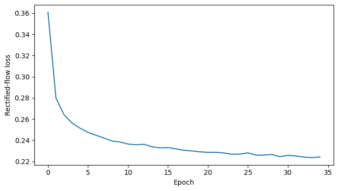
The loss curve is interpretable in the same spirit as the diffusion MSE: lower values usually indicate better local velocity prediction. Sampling quality also depends on the solver and on how accurately the learned field behaves along generated trajectories.
plt.figure(figsize=(7, 4))
plt.plot(image_history)
plt.xlabel("Epoch")
plt.ylabel("Rectified-flow loss")
plt.tight_layout()
plt.show()


@torch.no_grad()
def sample_rectified_flow(model, n_samples=16, steps=image_ode_steps, show_progress=True):
    model.eval()
    x = torch.randn(n_samples, image_channels, image_size, image_size, device=device)
    dt = 1.0 / steps
    iterator = range(steps)
    if show_progress:
        iterator = tqdm(iterator, desc="rectified-flow sampling", leave=False)

    for i in iterator:
        t = torch.full((n_samples, 1), i / steps, device=device)
        v = model(x, t)
        # A midpoint step is a simple but meaningful upgrade over raw Euler.
        x_mid = x + 0.5 * dt * v
        t_mid = torch.full((n_samples, 1), (i + 0.5) / steps, device=device)
        x = x + dt * model(x_mid, t_mid)

    x = x.clamp(-1.0, 1.0)
    return 0.5 * (x + 1.0).cpu()


image_samples = sample_rectified_flow(image_flow_model, n_samples=16)
image_grid = utils.make_grid(image_samples, nrow=4, pad_value=1.0)
plt.figure(figsize=(6, 6))
plt.imshow(image_grid.permute(1, 2, 0), cmap="gray")
plt.axis("off")
plt.show()
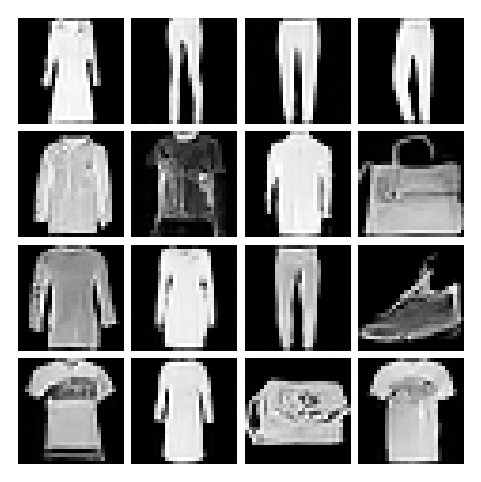
Midpoint integration introduces the engineering issue behind continuous-time generators. After training the field, sample quality depends on the ODE solver as well as on the network. Generation therefore combines local velocity prediction with global numerical integration.
Sampling, Evaluation, and Interpretation#
At image scale, evaluation follows the same distribution-level logic used for the earlier model families. Real and generated samples are compared in a pretrained feature space. Both sets should use the same preprocessing and moderate metric batches. Caching the real features avoids repeated work during solver or variant comparisons.
Warning
FID and KID require enough generated samples and the same real-data preprocessing pipeline used by the other image models. A poor score can come from undertraining, weak path design, insufficient solver accuracy, or too few samples in the estimate.
Note
At image scale, flow matching resembles diffusion architecturally: image tensors, time embeddings, U-Net-like processing, and regression losses. The predicted quantity is a transport velocity.
def prepare_for_inception_metrics(images):
    if images.size(1) == 1:
        images = images.repeat(1, 3, 1, 1)
    return images.clamp(0.0, 1.0)


@torch.no_grad()
def compute_rectified_flow_fid_and_kid(model, real_loader, device, num_samples=1000, metric_batch_size=32):
    fid = FrechetInceptionDistance(
        feature=2048,
        normalize=True,
        reset_real_features=False,
    ).set_dtype(torch.float64).to(device)
    kid = KernelInceptionDistance(
        feature=2048,
        subsets=10,
        subset_size=100,
        normalize=True,
        reset_real_features=False,
    ).to(device)

    seen_real = 0
    for real_images, _ in tqdm(real_loader, desc="Rectified-flow real metrics", leave=False):
        remaining = num_samples - seen_real
        if remaining <= 0:
            break
        real_images = real_images[: min(metric_batch_size, remaining)].to(device)
        real_images = 0.5 * (real_images + 1.0)
        real_images = prepare_for_inception_metrics(real_images)
        fid.update(real_images, real=True)
        kid.update(real_images, real=True)
        seen_real += real_images.size(0)

    generated = 0
    pbar = tqdm(total=num_samples, desc="rectified-flow fake metrics", leave=False)
    while generated < num_samples:
        batch_n = min(metric_batch_size, num_samples - generated)
        fake_images = sample_rectified_flow(
            model,
            n_samples=batch_n,
            steps=image_ode_steps,
            show_progress=False,
        ).to(device)
        fake_images = prepare_for_inception_metrics(fake_images)
        fid.update(fake_images, real=False)
        kid.update(fake_images, real=False)
        generated += batch_n
        pbar.update(batch_n)
    pbar.close()

    kid_mean, kid_std = kid.compute()
    return {
        "fid": fid.compute().item(),
        "kid_mean": kid_mean.item(),
        "kid_std": kid_std.item(),
    }


rectified_flow_metrics = compute_rectified_flow_fid_and_kid(
    image_flow_model,
    fashion_loader,
    device,
    num_samples=1000,
    metric_batch_size=32,
)
print(rectified_flow_metrics)
c:\Users\tivog\deep-generative-models\.venv\lib\site-packages\torchmetrics\utilities\prints.py:43: UserWarning: Metric `Kernel Inception Distance` will save all extracted features in buffer. For large datasets this may lead to large memory footprint.
  warnings.warn(*args, **kwargs)
{'fid': 30.816980599856606, 'kid_mean': 0.004778433125466108, 'kid_std': 0.0013600361999124289}
These numbers provide a quantitative distribution-level comparison. They should be read together with visual samples, solver analysis, and compute cost. A weak score can reflect architecture limits, undertraining, path design, or solver accuracy.
Flow matching expresses a central idea in modern generative modeling with unusual clarity: choose a geometric path from noise to data, learn the local motion along that path, and integrate the resulting field to generate samples.
In VAEs the geometry appears through latent variables and variational inference. In GANs it appears through the adversarial discrepancy. In diffusion it appears through the stochastic noising path. In flow matching it is written directly as a probability path with local velocity targets.