
Neural Network Foundations for Image Generation#
The goal of this chapter is not to offer a complete course on deep learning, but to isolate the pieces of neural network theory that are repeatedly used by modern generative models. A generative model for images typically combines function approximation, high-dimensional optimization, structured architectures, and representation learning. Even when the final probabilistic formulation looks sophisticated, the trainable components are still neural networks acting on tensors. If we do not understand why these networks are expressive, how they process spatial information, and why an autoencoder is already a nontrivial unsupervised model, later chapters become unnecessarily opaque.
We begin from the simplest viewpoint. A neural network is a parameterized function \(f_\theta\) obtained by composing affine maps with nonlinearities. The composition principle matters because each layer can be interpreted as a learned change of coordinates. When the input is an image, however, fully connected layers ignore the geometry of the pixel grid. This is why convolutional neural networks, and later U-Nets, became central in generative modeling: they encode locality, translation-aware feature extraction, and a hierarchy of receptive fields. Those architectural biases are not cosmetic. They reduce sample complexity and make the learned model behave in ways that better match images as structured objects.
Why This Chapter Matters for Generative Modeling#
It is tempting to skip quickly over neural-network preliminaries and move immediately to VAEs, GANs, or diffusion models. For a short seminar that choice might be acceptable. For a real course it is not. Every deep generative model is built from ordinary learnable components whose behavior we must understand well enough to trust their probabilistic interpretation. When a decoder outputs the parameters of a Gaussian distribution, it is still a neural network. When a discriminator distinguishes real from fake, it is still a neural network. When a diffusion model predicts noise, score, or velocity, it is still a neural network. If the student sees only the probabilistic wrapper and not the architectural engine underneath it, the whole subject risks looking more mysterious than it really is.
There is also a pedagogical reason to slow down here. Students coming from computer science often know that neural networks work in practice but have not reflected much on why certain architectures are repeatedly chosen. Students coming from mathematics may understand the formalism of optimization or probability but may not yet have an intuitive picture of what a convolution actually buys us. Students from less technical backgrounds may have seen images generated by modern AI systems but may still think of the network as an opaque black box. This chapter is therefore meant to give everyone a common vocabulary before the more specialized generative-model chapters begin.
From Perceptrons to Deep Feature Maps#
Consider an input vector \(\boldsymbol{x} \in \mathbb{R}^d\). A single hidden layer network computes
This formula already reveals the two ingredients that will remain with us for the whole course. The first is linear mixing through matrices such as \(\boldsymbol{W}_1\) and \(\boldsymbol{W}_2\). The second is the nonlinear activation \(\sigma\), without which the composition would collapse into another affine map. In practice, deep models alternate these operations many times and learn internal representations that become progressively more abstract.
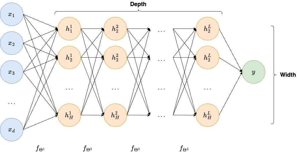
Fig. 7 The typical representation of a simple Multi-Layer Perceptron (MLP).#
For image generation, it is useful to remember that neural networks do not discover semantics by magic. They optimize a loss. What changes the nature of the learned representation is the learning problem. A classifier learns features that separate classes. An autoencoder learns features that preserve enough information to reconstruct the input. A denoising network learns features that are predictive of clean structure under corruption. Later chapters will exploit exactly this idea: one can shape a representation by changing the target task, even while keeping similar architectural ingredients.
Theorem 2 (Universal approximation in a form useful for intuition)
Let \(K \subset \mathbb{R}^d\) be compact and let \(g : K \to \mathbb{R}\) be continuous. For many standard non-polynomial activation functions \(\sigma\), a feedforward neural network with one hidden layer can approximate \(g\) uniformly on \(K\) with arbitrary precision.
Proof. A full proof is beyond the scope of this introductory chapter, but the statement can be justified by a density argument. One shows that finite linear combinations of ridge functions of the form \(\sigma(\boldsymbol{w}^\top \boldsymbol{x} + b)\) generate a function class that is dense in \(C(K)\) under the sup norm, provided \(\sigma\) is not a polynomial and satisfies mild regularity assumptions. The theorem does not claim that the approximation is easy to find, nor that the required width is small. Its value here is conceptual: neural networks are expressive enough in principle, so the real questions concern inductive bias, optimization, and data efficiency.
Convolutions, Locality, and Receptive Fields#
Images are arrays, not unordered vectors. A convolutional layer respects this structure by applying the same local filter at many positions. The weight sharing has two consequences. First, the number of parameters is reduced drastically when compared with a dense layer acting on the whole image. Second, the network becomes sensitive to local patterns regardless of where they occur. For classification this means edges, corners, and textures can be recognized across the field of view. For generation it means that local image statistics can be modeled in a coherent way.
If a stack of convolutional layers is deep enough, the effective receptive field grows, and the model can integrate local evidence into larger structures. This is one reason why modern generative models often combine downsampling and upsampling paths. Fine detail and global organization live at different scales. Architectures that preserve multi-scale information are therefore natural candidates for image synthesis.
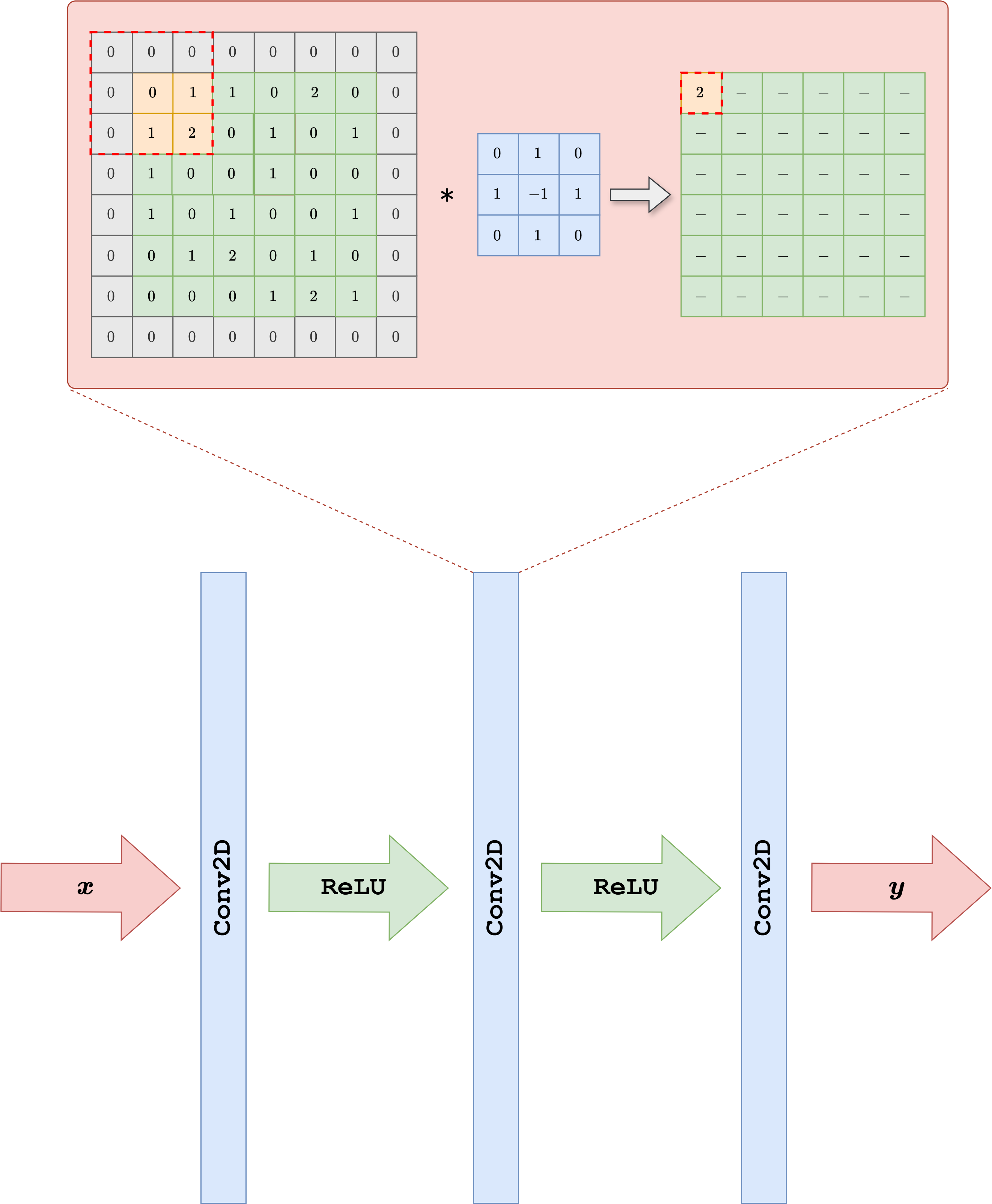
Fig. 8 A convolutional neural network used as a feature extractor. The same local processing idea will later reappear inside encoders, decoders, discriminators, and denoisers.#
The phrase receptive field deserves more emphasis than it usually receives in quick introductions. If the receptive field is too small, a network may faithfully detect local edges and textures but fail to organize them into a coherent object-level representation. If it is too large too early, the network may mix information too aggressively and lose fine detail. Generative modeling constantly negotiates this tradeoff because image synthesis requires both local realism and global coherence. A face generator must render pores, eyelashes, and hair strands, but it must also place those details consistently relative to eyes, nose, mouth, and head shape. A diffusion denoiser must clean local noise while preserving the large-scale semantic organization of the object. The architecture is therefore part of the modeling hypothesis, not just a computational container.
There is also a conceptual bridge here to probability. When we say that an architecture has a useful inductive bias, we mean that the class of functions it can represent efficiently aligns with the statistical regularities of the data. Convolutions assume that local patterns are meaningful and recur across positions. Pooling or downsampling assumes that some degree of coarse summary is acceptable at intermediate stages. Skip connections assume that information from earlier layers should sometimes survive almost unchanged into later stages. These are structural assumptions about natural images, expressed not in probabilistic notation but in network design.
Theorem 3 (Translation equivariance of discrete convolutions)
Let \(T_{\boldsymbol{\tau}}\) denote a discrete translation operator acting on an image by shifting it by \(\boldsymbol{\tau}\). If \(\mathcal{C}\) is a convolution with a fixed kernel and boundary effects are ignored, then
In other words, convolution is translation equivariant.
Proof. A discrete convolution computes each output pixel as the weighted sum of input pixels in a neighborhood determined by the kernel. If the whole input image is shifted by \(\boldsymbol{\tau}\), then the neighborhood seen at the translated location is exactly the translated version of the original neighborhood. Because the same kernel weights are reused at every position, the numerical combination performed after translation is identical to the original combination, only relocated by \(\boldsymbol{\tau}\). Therefore shifting first and convolving second gives the same result as convolving first and shifting second.
The theorem is elementary, but it explains one of the deepest reasons CNNs became standard for images. A learned edge detector should not need to relearn the same edge independently at every location in the image grid. Translation equivariance encodes this prior directly.
The U-Net as an Information-Preserving Architecture#
The U-Net architecture was originally introduced for image segmentation, yet it became one of the most important backbones in diffusion modeling. Its strength lies in the coexistence of two pathways. The contracting path builds abstract and spatially coarse features. The expanding path reconstructs fine spatial detail. Skip connections transfer intermediate features from encoder to decoder so that localization is not lost.
This architecture is especially suitable when the output should preserve much of the spatial organization of the input, as happens in denoising and conditional generation. A pure encoder-decoder with a severe bottleneck may discard detail too aggressively. A U-Net mitigates this issue by letting the decoder access multi-scale information directly. From the viewpoint of the later course, the U-Net is less a specific recipe than a structural principle: keep global context and local precision in communication.
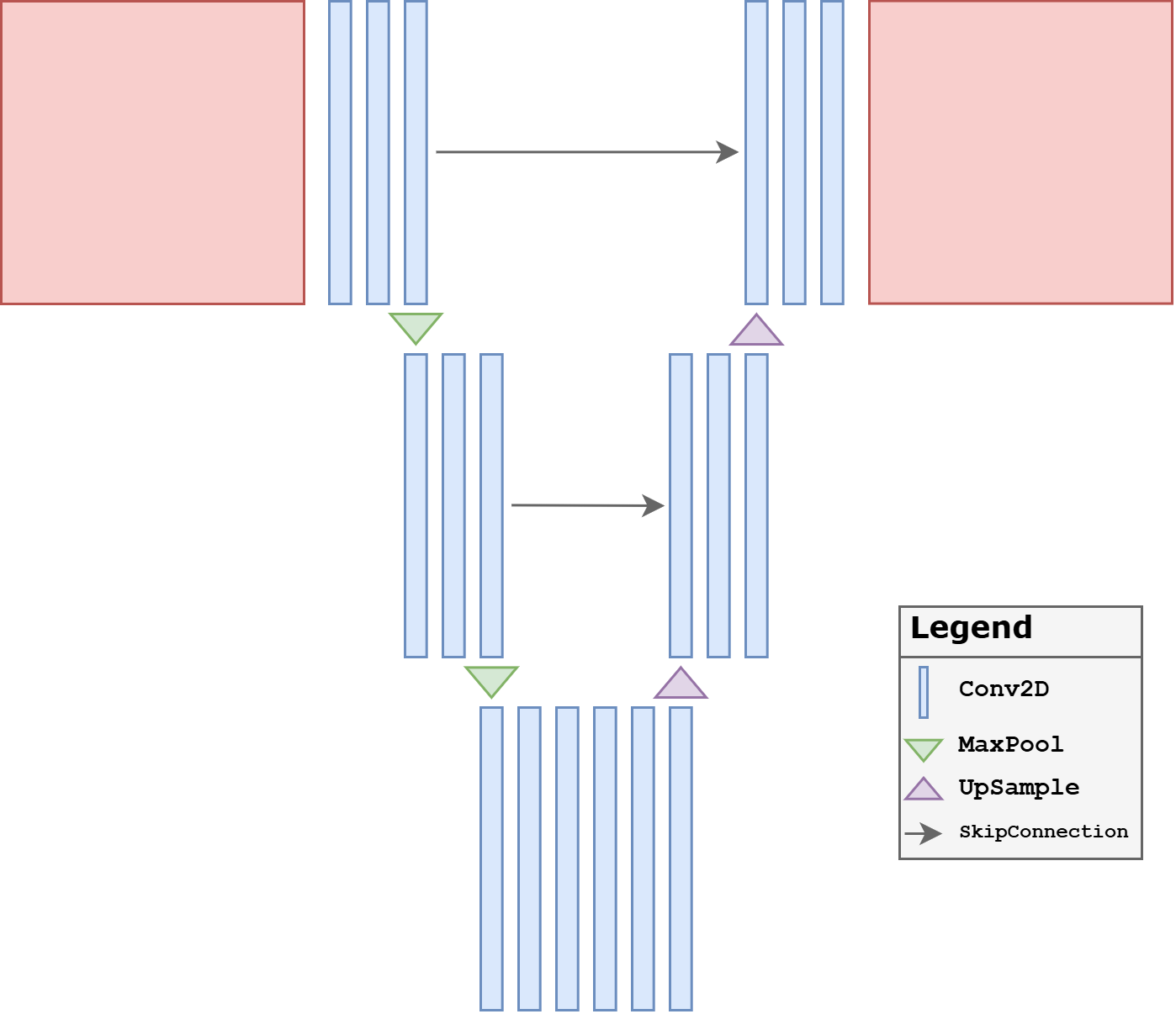
Fig. 9 A U-Net style architecture. In diffusion models, the input image is typically corrupted by noise and the network predicts either the noise, the score, or a related target.#
It is useful to compare the U-Net with a classical bottleneck autoencoder. In a strong bottleneck architecture, the network is forced to compress the entire input into a relatively small latent representation before reconstruction begins. This can be very useful when one wants the bottleneck itself to serve as a meaningful latent code, as in a variational autoencoder. In denoising, however, the goal is usually not to compress the whole image into a tiny representation. The goal is to modify the image while preserving its spatial identity. A denoiser benefits from remembering where structures are located. Skip connections provide exactly this memory.
For non-technical readers, one can imagine the U-Net as a system with two complementary views of the same image. One view zooms out and asks what global structure is present. The other view zooms back in and restores local detail, but it is allowed to consult the earlier high-resolution observations so that fine spatial information is not lost. This is why the architecture appears so naturally in diffusion and restoration tasks. The model repeatedly answers the question: given a partially corrupted image, what should remain and what should be corrected?
Unsupervised Learning and the Autoencoder Idea#
Before introducing probabilistic latent variable models, it is helpful to study the deterministic autoencoder. An encoder network maps \(\boldsymbol{x}\) to a latent code \(\boldsymbol{z} = e_\phi(\boldsymbol{x})\), while a decoder reconstructs the image through \(\widehat{\boldsymbol{x}} = d_\theta(\boldsymbol{z})\). Training often minimizes a reconstruction loss such as
The attractive idea is that a lower-dimensional latent space may capture the essential factors of variation. Yet, on its own, the deterministic autoencoder does not define a proper generative model unless we also specify how latent codes should be sampled. This observation is one of the conceptual bridges toward the variational autoencoder.
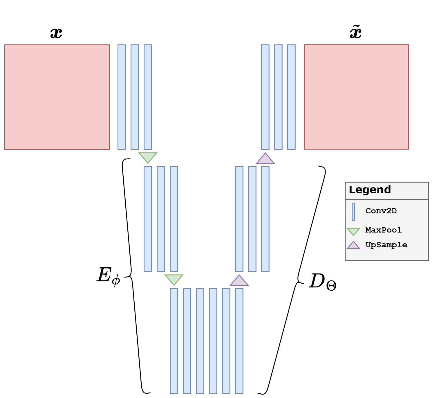
Fig. 10 The deterministic autoencoder suggests the latent-variable viewpoint but does not yet specify a probabilistic prior over latent codes.#
The limitation of the deterministic autoencoder should be stated carefully because it is conceptually important for the rest of the course. Suppose we train an excellent encoder-decoder pair with low reconstruction error. We may be tempted to say that we now have a generator: simply sample a latent code and decode it. But sample it from where. The deterministic training objective has not told us which latent codes are likely, which are impossible, or how mass should be distributed in latent space. Some codes may decode to meaningful images, others to nonsense, and nothing in the reconstruction objective alone resolves the ambiguity.
This is exactly where probabilistic latent-variable models enter the story. They keep the representational appeal of the autoencoder, namely the idea that images may be described through a lower-dimensional latent mechanism, but they add a probabilistic prior and an explicit generative interpretation. The VAE is therefore not an arbitrary variation on the autoencoder theme. It is the precise mathematical answer to the question that the deterministic autoencoder leaves open: how should latent space be organized so that sampling becomes meaningful.
The most important takeaway from this chapter is that the architectures used in deep generative models are not arbitrary containers for probability formulas. They encode assumptions about locality, scale, and information flow. When we later introduce encoders, decoders, discriminators, and denoisers, we shall reuse this architectural vocabulary rather than start from scratch each time. Students who want a broader deep learning background may consult the treatments in [GBC16] and [Bis06].