
Score-Based Models, SDEs, and Probability Flow ODEs#
When the number of diffusion steps becomes large and each corruption step becomes very small, the discrete noising chain is naturally rewritten in continuous time. The forward process is then described by a stochastic differential equation, and generation becomes the numerical solution of a reverse-time denoising dynamics. This formulation makes the geometry of diffusion models more explicit: the denoiser can be interpreted as a vector field that guides probability mass back toward the data distribution at every noise level.
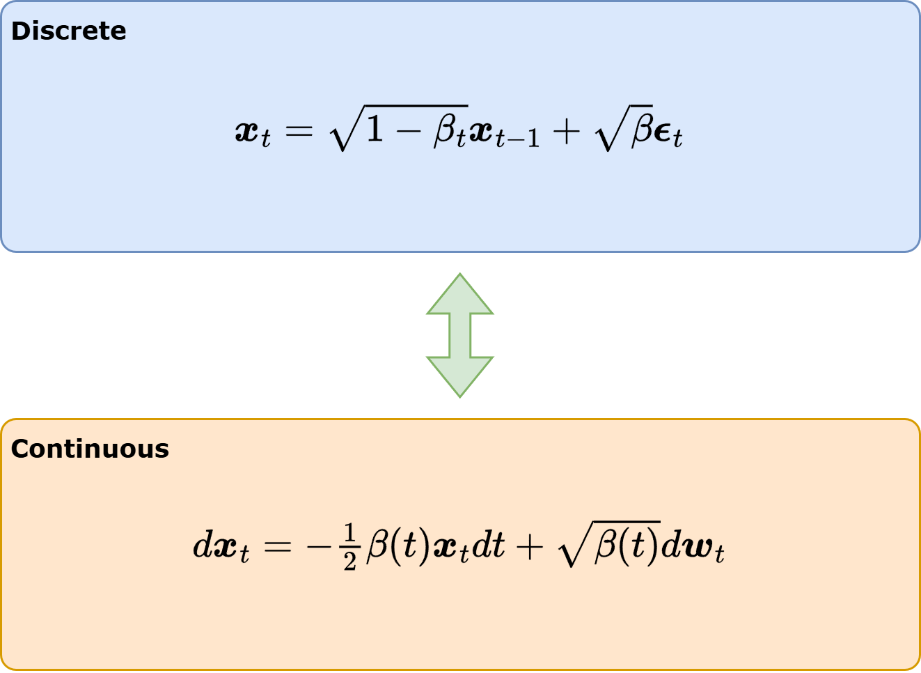
At the center of the discussion is the score field \(\nabla_{\boldsymbol{x}} \log p_t(\boldsymbol{x})\). In the discrete DDPM construction, the model is trained to predict the Gaussian perturbation added at time \(t\). In the continuous picture, the same prediction can be converted into a score, and that score can drive either a stochastic reverse-time SDE or a deterministic probability-flow ODE. The resulting theory explains why a single trained denoiser can support several different samplers while still being tied to the same family of marginals.
The continuous-time score-based formulation used here follows Song et al. [SSDK+21], while the denoising-score-matching bridge goes back to Song and Ermon [SE20].
A pretrained FashionMNIST DDPM denoiser can therefore be reused almost verbatim. The main extra ingredients are the score conversion formula, the interpretation of the discrete schedule as a continuous variance-preserving path, and the choice of numerical solver. Once these ingredients are in place, ancestral DDPM sampling, reverse-SDE sampling, and probability-flow ODE sampling appear as different discretizations of one underlying denoising geometry.
Important
A pretrained noise predictor already contains a score model. Continuous-time diffusion is the language that makes this statement precise.
ODEs, SDEs, and Continuous-Time Trajectories#
An ordinary differential equation such as
assigns a velocity vector to every point of space and every time instant. Once an initial condition is fixed, the equation determines an entire trajectory \(t \mapsto \boldsymbol{x}(t)\). The sample does not jump arbitrarily from one location to another. It moves by following the vector field prescribed by \(\boldsymbol{f}\). This is the most basic continuous-time picture of generation: start from some initial state and let a learned dynamics transport it through space.
The geometric viewpoint matters because it turns generation into a problem of designing trajectories. If the vector field points in sensible directions, the path remains coherent and gradually approaches the region of interest. If the vector field is poor, the trajectory drifts into implausible configurations. In this sense, an ODE already contains the seed of a generative model: it gives a rule for how samples move over time.
A pure ODE, however, is often too rigid for a noising process. If the goal is to spread the data distribution until it becomes close to a simple Gaussian reference, deterministic motion alone is usually not enough. This is why diffusion models move from ODEs to stochastic differential equations:
where \(\boldsymbol{w}\) is Brownian motion. The drift \(\boldsymbol{f}\) provides systematic motion, while the diffusion coefficient \(g(t)\) injects randomness continuously over time.
The interpretation changes in an important way. A trajectory is no longer fixed by its initial condition alone. Once stochasticity is added, the model defines a distribution over trajectories. This is exactly the right language for a noising process: two samples starting from the same clean image can follow different corrupted paths, while still sharing the same one-time marginals. Diffusion models live in this intermediate territory: the forward process is stochastic, while some reverse processes remain stochastic and others can be rewritten as deterministic flows with the same marginals.
Numerical Example: A One-Dimensional Score
Suppose that at some noise level the marginal density were a Gaussian centered at \(2\) with unit variance. Then
If the current sample is \(x=5\), the score is \(-3\), so the vector field points left, toward the high-density region. If the current sample is \(x=0\), the score is \(2\), so the vector field points right. The score does not report the density value itself. It reports the local direction in which the sample should move to become more probable.
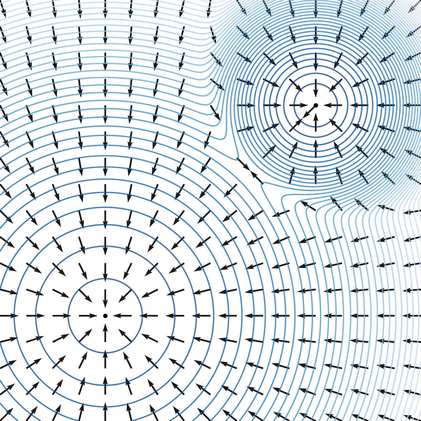
Fig. 41 The score field \(\nabla_{\boldsymbol{x}}\log p_t(\boldsymbol{x})\) points toward regions of higher probability under the current noisy marginal. The contour lines represent level sets of the density, while the arrows show the local direction in which probability increases most rapidly. In high-dimensional image models the same object is not drawn explicitly, but the denoiser is trained to approximate this direction at every noise level.#
The language of ODEs and SDEs is therefore not a change of topic. It is the natural way of expressing what the diffusion model has been doing all along in discrete time: construct a family of progressively noisier distributions, then learn a reverse dynamics that brings samples back toward the data manifold.
The Diffusion SDE: the Variance-Preserving Process as a Continuous-Time Limit#
The continuous-time process can be obtained directly from the DDPM forward chain by letting the number of steps grow. Recall the forward update from the previous chapter, which corrupts the clean image through the recursion
where \(\beta_k\in(0,1)\) is the per-step variance and the perturbations \(\boldsymbol{\varepsilon}_k\) are independent across steps. This is a discrete dynamical system indexed by the integer step \(k\in\{1,\dots,N\}\). We now study what the recursion becomes when the number of steps \(N\) grows without bound while each individual step becomes correspondingly smaller.
The first move is to rescale the step index into a continuous time variable. Let \(t = k/N \in [0,1]\) and write \(\Delta t = 1/N\), so that consecutive steps are separated by a small time increment \(\Delta t\). The discrete schedule \(\{\beta_k\}\) is reparameterized through a smooth function \(\beta(t)\) by setting
This is the key modeling choice: the per-step variance is proportional to the time increment. Under this scaling the accumulated noise remains finite as \(\Delta t\to 0\), neither vanishing nor diverging. Substituting it into the recursion gives
Since \(\Delta t\) is small, we expand the signal coefficient to first order,
and, keeping only the leading terms, obtain
The two terms on the right have a different character. The first is deterministic and proportional to \(\Delta t\); it is an ordinary drift that contracts the signal toward the origin. The second is stochastic and proportional to \(\sqrt{\Delta t}\), the characteristic scaling of a Brownian increment: if \(\boldsymbol{w}(t)\) denotes a standard Brownian motion, then \(\boldsymbol{w}(t+\Delta t)-\boldsymbol{w}(t)\) is Gaussian with covariance \(\Delta t\,\boldsymbol{I}\), so the term \(\sqrt{\Delta t}\,\boldsymbol{\varepsilon}(t)\) has the law of the infinitesimal increment \(d\boldsymbol{w}\). Taking \(\Delta t\to 0\) turns the recursion into the variance-preserving SDE
This SDE is the continuous-time form of the DDPM forward process. The DDPM forward chain is its Euler-Maruyama discretization on the uniform grid \(t_k = k/N\), with per-step variance \(\beta_k = \beta(t_{k-1})\Delta t\). The drift \(-\tfrac12\beta(t)\boldsymbol{x}\) damps the signal, while the diffusion term \(\sqrt{\beta(t)}\,d\boldsymbol{w}\) injects Gaussian noise at every instant. The name variance-preserving reflects the balance between these two effects: the same schedule \(\beta(t)\) ties the attenuation of the signal to the injection of noise, so that the total variance stays under control along the path.
The same limit yields the closed-form forward marginal that made DDPM training tractable. Define the continuous cumulative retention factor
the continuous-time form of the finite product \(\prod_{s\le k}(1-\beta_s)\) from the DDPM chapter. The correspondence is again a small-step expansion, since
With this factor the marginal of the VP-SDE is Gaussian,
the continuous analogue of the DDPM forward marginal \(\boldsymbol{x}_k=\sqrt{\alpha_k}\,\boldsymbol{x}_0+\sqrt{1-\alpha_k}\,\boldsymbol{\varepsilon}\), with the signal-retention factor now a smooth function of time instead of a finite product of stepwise coefficients [HJA20, SSDK+21].
The behavior along the path matches the discrete picture. At early times the sample still looks strongly tied to the original image, while at late times the Gaussian term dominates and the state becomes nearly pure noise. Continuous time turns that progression into a smooth deformation of distributions, and makes available the full apparatus of stochastic calculus for describing the reverse, generative direction.
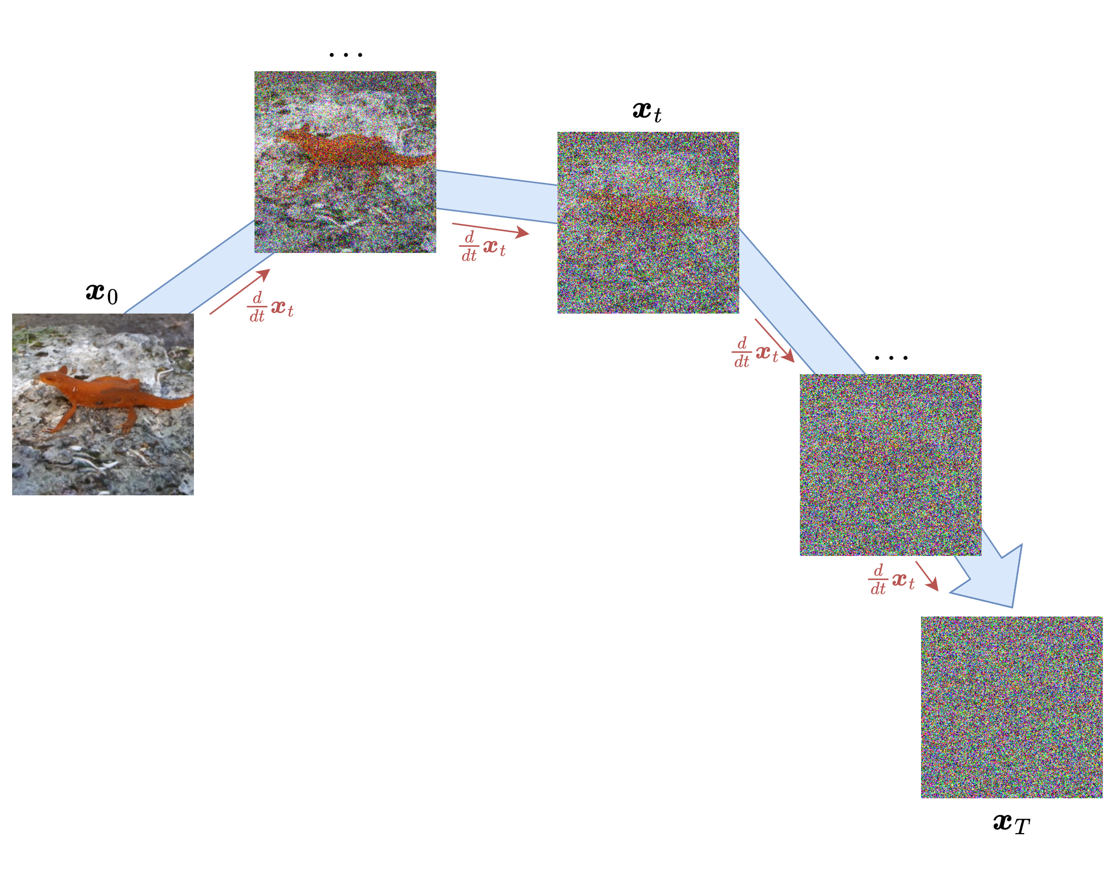
Fig. 42 The variance-preserving SDE gives a continuous-time view of the same corruption geometry used by DDPMs. The signal coefficient is controlled by the cumulative factor \(\alpha(t)\), while the stochastic term progressively injects Gaussian noise.#
Theorem 16 (VP-SDE forward marginal)
For the variance-preserving SDE,
the conditional law of \(\boldsymbol{x}_t\) given \(\boldsymbol{x}_0\) is Gaussian with
Reverse-Time Dynamics, Score Learning, and Denoising Score Matching#
The forward VP-SDE tells how data are progressively corrupted. Generation requires the opposite direction: start from a simple noisy distribution and move backward toward the data. For a generic forward diffusion
it can be proved that the reverse-time SDE becomes:
This is the first place where the score enters naturally. It describes the energy price we must pay for reducing the entropy of the process. The reverse dynamics combine the forward drift correction with the gradient of the log-density of the current noisy marginal. That gradient tells the sample in which local direction probability mass increases.
For the VP family this becomes
If the score were known exactly, simulating this reverse SDE would already yield a generative algorithm. The real learning problem is therefore to approximate the score field well enough that the reverse dynamics become usable in practice.
This is where denoising score matching enters. In the VP setting, the forward perturbation law is explicit:
Because this perturbation is known, the conditional score of the noisy variable given the clean sample is also explicit. The intractable score of the noisy-data marginal is therefore replaced by a supervised regression target manufactured by the forward diffusion itself. Conceptually, this is extremely close to DDPM training: the corruption process is chosen precisely so that it produces a tractable denoising target.
A neural network can therefore be trained to approximate the score field at each noise level,
The VP perturbation law makes this feasible by providing analytic access to the local denoising target. The score network is learned indirectly through the corruption mechanism itself, without estimating the unknown density \(p_t\) directly.
In the VP formulation, the denoising-score-matching objective can be written directly in terms of the diffusion perturbation. At a fixed time level \(t\), the known conditional score is
Training against this target yields the score of the noisy marginal at that time level.
Theorem 17 (VP denoising score matching recovers the noisy-marginal score)
At a fixed noise level \(t\), consider the VP perturbation
The minimizer of
is the score of the noisy marginal:
Proof. Condition on \(\boldsymbol{x}_t\). The optimal regression target is the conditional expectation of the known Gaussian target:
For the VP perturbation, the conditional target above is exactly the score of the noisy marginal. Indeed, differentiating the noisy density obtained by marginalizing over \(\boldsymbol{x}_0\) yields the standard denoising-score-matching identity
Therefore the minimizer of the regression objective is precisely the score of the noisy marginal.
This is the continuous-time analogue of what happened in DDPM training. The generative problem is not attacked by estimating a high-dimensional density directly. It is attacked by constructing a diffusion perturbation whose conditional score is explicit enough to manufacture a supervised target. Once that target is available, score estimation becomes a denoising regression problem indexed by time.
From Reverse SDE Sampling to a Pretrained DDPM Denoiser#
If a score approximation \(\boldsymbol{s}_\theta\) is available, the reverse VP-SDE can be simulated numerically. Over a small backward interval of length \(\Delta t\), an Euler-Maruyama step takes the form
This is the continuous-time ancestor of diffusion sampling. The model repeatedly estimates how the current noisy sample should move toward higher probability and then injects the stochastic correction required by the reverse diffusion law. In discrete diffusion language, this is the logic behind ancestral sampling.
The crucial practical point is that one does not need to train a second network specifically for this chapter. The denoiser learned in the DDPM notebook already contains the relevant information. A pretrained noise predictor can be turned into a score model and, through the same identity, into an estimator of the clean image hidden underneath the current noisy state.
The abstract score-network discussion becomes concrete once one reuses the denoiser from the discrete DDPM model. Suppose the network has been trained in the usual noise-prediction form, so that
For the VP perturbation path, the Gaussian conditional score is known in closed form. This makes it possible to convert the noise predictor into a score predictor with an explicit formula. It also yields a reconstruction formula for the clean image hidden inside \(\boldsymbol{x}_t\), which is the diffusion-model incarnation of Tweedie’s formula: once the score of the noisy marginal is known, one can estimate the underlying clean signal.
Theorem 18 (Score, clean-image reconstruction, and a pretrained noise predictor)
For the variance-preserving forward marginal,
In the discrete DDPM notation this becomes
Equivalently, the clean-image estimate can be written as
This is the diffusion-style form of Tweedie’s formula.
Proof. The Gaussian forward conditional satisfies
Using
one gets
Replacing the unknown noise by the neural estimate gives the score formula.
Now solve the forward marginal identity
for \(\boldsymbol{x}_0\) and substitute either the predicted noise or the score formula. This gives
The second expression is the Tweedie-style reconstruction formula written in diffusion notation.
This identity is the exact bridge from the previous notebook to the current one. Once a DDPM denoiser has been trained, the score field is already present implicitly inside the noise predictor. The same formula also explains why diffusion samplers repeatedly build \(\hat{\boldsymbol{x}}_{0|t}\): they are using the score of the noisy marginal to infer the cleaner configuration hidden underneath the current sample.
The Probability-Flow ODE and Its Deterministic Discretization#
The same marginals also admit a deterministic dynamics. Song et al. showed that removing the stochastic term yields the probability-flow ODE:
For the VP family this becomes
The one-time marginals of this ODE agree with those of the reverse-time SDE, but the trajectories are deterministic. This is the continuous-time object that sits behind deterministic diffusion samplers such as DDIM [SME21, SSDK+21].
Once the PF-ODE is available, sampling becomes a numerical-integration problem. The simplest option is a first-order scheme: over a short interval one freezes the vector field at the current point and advances with an Euler step. In backward time this means
Unlike the reverse SDE discretization, there is no fresh Gaussian perturbation. The same initial terminal noise therefore always produces the same trajectory. This deterministic viewpoint is precisely what makes the connection with DDIM so clean. In practice, the PF-ODE interpretation turns diffusion sampling into a standard solver problem: once the score is available, sample quality depends on the numerical integrator used to traverse the learned denoising field.
The DDIM update can then be read as a particularly natural first-order deterministic solver expressed in the familiar variables \(\hat{\boldsymbol{x}}_{0|t}\) and \(\boldsymbol{\varepsilon}_\theta\). Instead of injecting fresh noise, the algorithm follows the denoising field implied by the current estimate of the clean image and moves directly to a less noisy point on the same probability path.
Theorem 19 (Probability-flow ODE discretizes to deterministic DDIM)
Consider the VP family and assume the denoiser provides a noise estimate \(\boldsymbol{\varepsilon}_\theta(\boldsymbol{x}_t,t)\) together with the implied clean-image estimate
If one advances from time \(t\) to an earlier time \(t' < t\) by the deterministic update
then the resulting scheme is exactly DDIM with \(\eta = 0\). Moreover, if the probability-flow ODE is integrated over the interval \([t',t]\) while freezing the denoiser output on that interval, the resulting integral update is exactly the deterministic DDIM step. Consequently, once \(\boldsymbol{x}_T\) is fixed, the whole DDIM trajectory is fixed.
Proof. The first statement is immediate: the displayed update is the deterministic DDIM rule, written with continuous-time notation \(\alpha(t)\) instead of a discrete index. Because no fresh Gaussian perturbation is injected, every iterate is a deterministic function of the previous one. Fixing \(\boldsymbol{x}_T\) therefore fixes the whole trajectory.
To connect this update to the probability-flow ODE, write on the interval \([t',t]\)
where the denoiser output is frozen at its value computed from \((\boldsymbol{x}_t,t)\). Since
differentiating gives
Now use the score conversion formula
and the decomposition
Substituting both identities yields
which is exactly the VP probability-flow ODE with the learned score in place of the exact one.
Integrating this ODE from \(t\) backward to \(t'\) gives
Because \(\widetilde{\boldsymbol{x}}(\tau)\) was constructed so that its derivative is exactly the integrand, the fundamental theorem of calculus gives
This is precisely the deterministic DDIM update.
Equivalently, one may view the argument as a one-step discretization of the PF-ODE in which the denoiser output is held constant across the interval and the resulting integral is evaluated in closed form through the coefficients \(\sqrt{\alpha(\tau)}\) and \(\sqrt{1-\alpha(\tau)}\). Therefore deterministic DDIM is the natural finite-step integral solver associated with the VP probability-flow ODE.
The continuous formulation therefore organizes several samplers around a single learned field. The VP-SDE explains the forward corruption law. The reverse-time SDE gives a stochastic denoising sampler whose finite-step version is ancestral DDPM. The probability-flow ODE gives a deterministic denoising sampler whose finite-step version is DDIM with \(\eta = 0\). What changes from one algorithm to another is the numerical path; the learned denoiser and the underlying probability family remain the same.
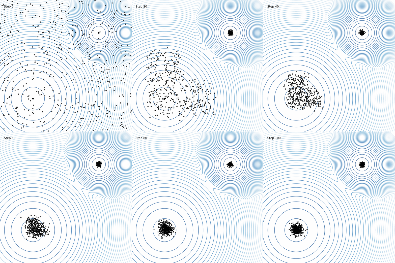
Fig. 43 A sampling trajectory follows the learned denoising field from a noisy initial condition toward the data region. Reverse-SDE samplers add stochastic perturbations along the way, while probability-flow ODE samplers follow a deterministic path once the terminal noise is fixed. The common ingredient is the same score information supplied by the trained denoiser.#
Discrete and Continuous Diffusion: A Dictionary#
After the forward SDE, reverse-time SDE, probability-flow ODE, and DDIM connection have been introduced, the discrete and continuous languages can be placed side by side. The table below summarizes the correspondence used throughout the chapter.
Discrete DDPM language |
Continuous SDE language |
Meaning |
|---|---|---|
Time index \(t \in \{1,\ldots,T\}\) |
Time variable \(t \in [0,1]\) |
Position along the noising path |
Per-step variance \(\beta_t\) |
Noise rate \(\beta(t)\) |
Strength of the local corruption |
One-step retention \(\bar{\alpha}_t = 1-\beta_t\) |
Infinitesimal signal decay in the VP drift |
Local signal attenuation |
Cumulative retention \(\alpha_t = \prod_{s=1}^t \bar{\alpha}_s\) |
Cumulative retention \(\alpha(t)=\exp\left(-\int_0^t \beta(s)\,ds\right)\) |
Amount of clean-image signal still present |
Forward transition \(q(\boldsymbol{x}_t | \boldsymbol{x}_{t-1})\) |
Forward SDE \(d\boldsymbol{x}=\boldsymbol{f}(\boldsymbol{x},t)\,dt+g(t)\,d\boldsymbol{w}\) |
Rule that corrupts data into noise |
Learned reverse kernel \(p_\theta(\boldsymbol{x}_{t-1} | \boldsymbol{x}_t)\) |
Reverse-time SDE |
Stochastic denoising dynamics |
Deterministic DDIM, \(\eta=0\) |
Probability-flow ODE |
Deterministic denoising dynamics with the same one-time marginals |
Noise predictor \(\boldsymbol{\varepsilon}_\theta\) |
Score field \(\boldsymbol{s}_\theta \approx \nabla_{\boldsymbol{x}}\log p_t(\boldsymbol{x})\) |
Two parameterizations of the same denoising information under the VP marginal |
This dictionary is useful because the implementation reuses a discrete DDPM denoiser while interpreting its predictions through continuous-time equations. The symbols change, but the learned denoising information is the same.
Using the FashionMNIST DDPM Denoiser as a Score Network#
The implementation below uses the same FashionMNIST denoiser trained in the DDPM notebook. The network architecture, time embedding, and discrete schedule are kept identical. After loading the weights, the score is obtained through the theorem above, and the resulting field is used to run three samplers on the same model:
the ancestral DDPM sampler;
an Euler-Maruyama reverse-SDE sampler;
a probability-flow ODE sampler.
Because all three samplers are driven by the same denoiser, the comparison is about the geometry of the reverse dynamics rather than about differences in training.
This reuse of a pretrained DDPM denoiser follows directly from the relationship between noise prediction and score prediction highlighted by [SSDK+21].
Loading the Pretrained DDPM Denoiser#
import math
from pathlib import Path

import matplotlib.pyplot as plt
import torch
import torch.nn as nn
import torch.nn.functional as F
from torch.utils.data import DataLoader
from torchmetrics.image.fid import FrechetInceptionDistance
from torchmetrics.image.kid import KernelInceptionDistance
from torchvision import datasets, transforms, utils
from tqdm.auto import tqdm

device = torch.device("cuda" if torch.cuda.is_available() else "cpu")
torch.manual_seed(7)
if device.type == "cuda":
    torch.cuda.manual_seed_all(7)

project_root = Path.cwd() if (Path.cwd() / "_config.yml").exists() else Path.cwd().parent
artifacts_dir = project_root / "artifacts"
artifacts_dir.mkdir(exist_ok=True)
ddpm_checkpoint_path = artifacts_dir / "ddpm_fashionmnist.pt"

batch_size = 128
metric_batch_size = 64
num_workers = 0
image_size = 28
channels = 1
base_channels = 64
time_dim = 128
timesteps = 300

transform = transforms.Compose([
    transforms.ToTensor(),
    transforms.Lambda(lambda x: 2.0 * x - 1.0),
])

test_dataset = datasets.FashionMNIST(root=project_root / "data", train=False, download=True, transform=transform)
test_loader = DataLoader(
    test_dataset,
    batch_size=batch_size,
    shuffle=False,
    num_workers=num_workers,
    pin_memory=(device.type == "cuda"),
)
betas = torch.linspace(1e-4, 0.02, timesteps, device=device)
bar_alphas = 1.0 - betas
alphas = torch.cumprod(bar_alphas, dim=0)
alphas_prev = torch.cat([torch.tensor([1.0], device=device), alphas[:-1]], dim=0)

sqrt_alphas = torch.sqrt(alphas)
sqrt_one_minus_alphas = torch.sqrt(1.0 - alphas)
sqrt_recip_bar_alphas = torch.sqrt(1.0 / bar_alphas)
posterior_variance = betas * (1.0 - alphas_prev) / (1.0 - alphas)


def extract(coefficients, t, x_shape):
    out = coefficients.gather(0, t)
    return out.view(t.shape[0], *((1,) * (len(x_shape) - 1)))
class SinusoidalTimeEmbedding(nn.Module):
    def __init__(self, dim):
        super().__init__()
        self.dim = dim

    def forward(self, t):
        half_dim = self.dim // 2
        factor = math.log(10000.0) / max(half_dim - 1, 1)
        frequencies = torch.exp(torch.arange(half_dim, device=t.device) * -factor)
        angles = t.float().unsqueeze(1) * frequencies.unsqueeze(0)
        embedding = torch.cat([angles.sin(), angles.cos()], dim=1)
        if self.dim % 2 == 1:
            embedding = F.pad(embedding, (0, 1))
        return embedding


class ResidualBlock(nn.Module):
    def __init__(self, in_channels, out_channels, time_dim):
        super().__init__()
        self.conv1 = nn.Conv2d(in_channels, out_channels, kernel_size=3, padding=1)
        self.conv2 = nn.Conv2d(out_channels, out_channels, kernel_size=3, padding=1)
        self.time_mlp = nn.Linear(time_dim, out_channels)
        self.norm1 = nn.GroupNorm(8, out_channels)
        self.norm2 = nn.GroupNorm(8, out_channels)
        self.activation = nn.SiLU()
        self.residual = (
            nn.Conv2d(in_channels, out_channels, kernel_size=1)
            if in_channels != out_channels else nn.Identity()
        )

    def forward(self, x, t_emb):
        h = self.conv1(x)
        h = self.norm1(h)
        h = self.activation(h)

        # Broadcast the time embedding across spatial positions.
        time_term = self.time_mlp(t_emb).unsqueeze(-1).unsqueeze(-1)
        h = h + time_term

        h = self.conv2(h)
        h = self.norm2(h)
        h = self.activation(h)
        return h + self.residual(x)


class SmallUNet(nn.Module):
    def __init__(self, in_channels=1, base_channels=64, time_dim=128):
        super().__init__()
        self.time_embedding = nn.Sequential(
            SinusoidalTimeEmbedding(time_dim),
            nn.Linear(time_dim, time_dim),
            nn.SiLU(),
            nn.Linear(time_dim, time_dim),
        )

        self.input_conv = nn.Conv2d(in_channels, base_channels, kernel_size=3, padding=1)

        self.down1 = ResidualBlock(base_channels, base_channels, time_dim)
        self.downsample1 = nn.Conv2d(base_channels, base_channels * 2, kernel_size=4, stride=2, padding=1)
        self.down2 = ResidualBlock(base_channels * 2, base_channels * 2, time_dim)
        self.downsample2 = nn.Conv2d(base_channels * 2, base_channels * 4, kernel_size=4, stride=2, padding=1)
        self.down3 = ResidualBlock(base_channels * 4, base_channels * 4, time_dim)

        self.mid = ResidualBlock(base_channels * 4, base_channels * 4, time_dim)

        self.upsample2 = nn.ConvTranspose2d(base_channels * 4, base_channels * 2, kernel_size=4, stride=2, padding=1)
        self.up2 = ResidualBlock(base_channels * 4, base_channels * 2, time_dim)
        self.upsample1 = nn.ConvTranspose2d(base_channels * 2, base_channels, kernel_size=4, stride=2, padding=1)
        self.up1 = ResidualBlock(base_channels * 2, base_channels, time_dim)
        self.output_conv = nn.Conv2d(base_channels, in_channels, kernel_size=1)

    def forward(self, x, t):
        t_emb = self.time_embedding(t)

        # Save an early feature map so the decoder can recover detail later.
        x0 = self.input_conv(x)
        x1 = self.down1(x0, t_emb)
        x2 = self.downsample1(x1)
        x2 = self.down2(x2, t_emb)
        x3 = self.downsample2(x2)
        x3 = self.down3(x3, t_emb)

        x_mid = self.mid(x3, t_emb)

        x_up = self.upsample2(x_mid)
        x_up = torch.cat([x_up, x2], dim=1)
        x_up = self.up2(x_up, t_emb)
        x_up = self.upsample1(x_up)
        # Skip connection joins coarse semantics with finer spatial detail.
        x_up = torch.cat([x_up, x1], dim=1)
        x_up = self.up1(x_up, t_emb)
        return self.output_conv(x_up)

model = SmallUNet(in_channels=channels, base_channels=base_channels, time_dim=time_dim).to(device)
if not ddpm_checkpoint_path.exists():
    raise FileNotFoundError(f"Missing DDPM weights at {ddpm_checkpoint_path}. Run the discrete diffusion notebook first.")
model.load_state_dict(torch.load(ddpm_checkpoint_path, map_location=device))
model.eval()
#
SmallUNet(
  (time_embedding): Sequential(
    (0): SinusoidalTimeEmbedding()
    (1): Linear(in_features=128, out_features=128, bias=True)
    (2): SiLU()
    (3): Linear(in_features=128, out_features=128, bias=True)
  )
  (input_conv): Conv2d(1, 64, kernel_size=(3, 3), stride=(1, 1), padding=(1, 1))
  (down1): ResidualBlock(
    (conv1): Conv2d(64, 64, kernel_size=(3, 3), stride=(1, 1), padding=(1, 1))
    (conv2): Conv2d(64, 64, kernel_size=(3, 3), stride=(1, 1), padding=(1, 1))
    (time_mlp): Linear(in_features=128, out_features=64, bias=True)
    (norm1): GroupNorm(8, 64, eps=1e-05, affine=True, bias=True)
    (norm2): GroupNorm(8, 64, eps=1e-05, affine=True, bias=True)
    (activation): SiLU()
    (residual): Identity()
  )
  (downsample1): Conv2d(64, 128, kernel_size=(4, 4), stride=(2, 2), padding=(1, 1))
  (down2): ResidualBlock(
    (conv1): Conv2d(128, 128, kernel_size=(3, 3), stride=(1, 1), padding=(1, 1))
    (conv2): Conv2d(128, 128, kernel_size=(3, 3), stride=(1, 1), padding=(1, 1))
    (time_mlp): Linear(in_features=128, out_features=128, bias=True)
    (norm1): GroupNorm(8, 128, eps=1e-05, affine=True, bias=True)
    (norm2): GroupNorm(8, 128, eps=1e-05, affine=True, bias=True)
    (activation): SiLU()
    (residual): Identity()
  )
  (downsample2): Conv2d(128, 256, kernel_size=(4, 4), stride=(2, 2), padding=(1, 1))
  (down3): ResidualBlock(
    (conv1): Conv2d(256, 256, kernel_size=(3, 3), stride=(1, 1), padding=(1, 1))
    (conv2): Conv2d(256, 256, kernel_size=(3, 3), stride=(1, 1), padding=(1, 1))
    (time_mlp): Linear(in_features=128, out_features=256, bias=True)
    (norm1): GroupNorm(8, 256, eps=1e-05, affine=True, bias=True)
    (norm2): GroupNorm(8, 256, eps=1e-05, affine=True, bias=True)
    (activation): SiLU()
    (residual): Identity()
  )
  (mid): ResidualBlock(
    (conv1): Conv2d(256, 256, kernel_size=(3, 3), stride=(1, 1), padding=(1, 1))
    (conv2): Conv2d(256, 256, kernel_size=(3, 3), stride=(1, 1), padding=(1, 1))
    (time_mlp): Linear(in_features=128, out_features=256, bias=True)
    (norm1): GroupNorm(8, 256, eps=1e-05, affine=True, bias=True)
    (norm2): GroupNorm(8, 256, eps=1e-05, affine=True, bias=True)
    (activation): SiLU()
    (residual): Identity()
  )
  (upsample2): ConvTranspose2d(256, 128, kernel_size=(4, 4), stride=(2, 2), padding=(1, 1))
  (up2): ResidualBlock(
    (conv1): Conv2d(256, 128, kernel_size=(3, 3), stride=(1, 1), padding=(1, 1))
    (conv2): Conv2d(128, 128, kernel_size=(3, 3), stride=(1, 1), padding=(1, 1))
    (time_mlp): Linear(in_features=128, out_features=128, bias=True)
    (norm1): GroupNorm(8, 128, eps=1e-05, affine=True, bias=True)
    (norm2): GroupNorm(8, 128, eps=1e-05, affine=True, bias=True)
    (activation): SiLU()
    (residual): Conv2d(256, 128, kernel_size=(1, 1), stride=(1, 1))
  )
  (upsample1): ConvTranspose2d(128, 64, kernel_size=(4, 4), stride=(2, 2), padding=(1, 1))
  (up1): ResidualBlock(
    (conv1): Conv2d(128, 64, kernel_size=(3, 3), stride=(1, 1), padding=(1, 1))
    (conv2): Conv2d(64, 64, kernel_size=(3, 3), stride=(1, 1), padding=(1, 1))
    (time_mlp): Linear(in_features=128, out_features=64, bias=True)
    (norm1): GroupNorm(8, 64, eps=1e-05, affine=True, bias=True)
    (norm2): GroupNorm(8, 64, eps=1e-05, affine=True, bias=True)
    (activation): SiLU()
    (residual): Conv2d(128, 64, kernel_size=(1, 1), stride=(1, 1))
  )
  (output_conv): Conv2d(64, 1, kernel_size=(1, 1), stride=(1, 1))
)
Reconstructing \(\hat{\boldsymbol{x}}_{0|t}\) and the Score Field#
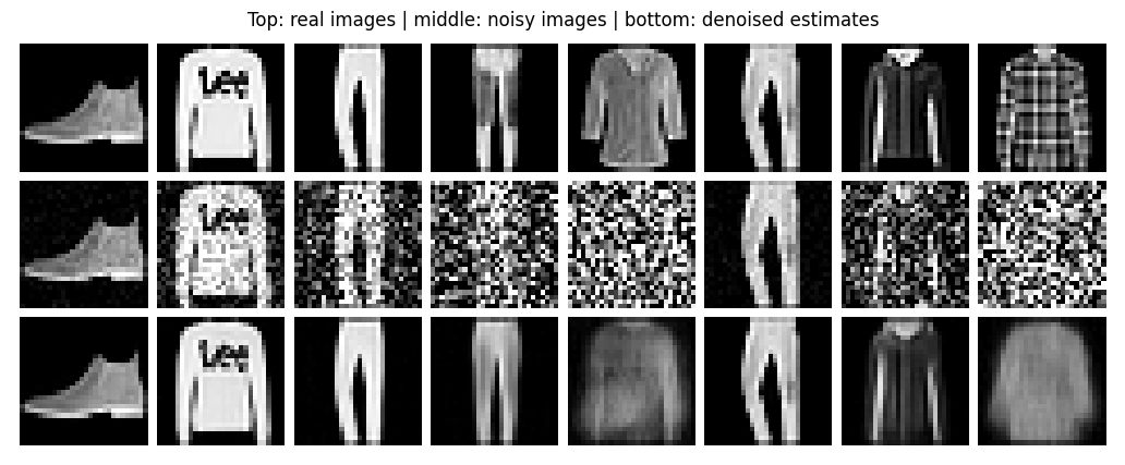
The easiest place to see the score interpretation in action is to start from a real image, corrupt it at a chosen time, and then reconstruct the clean image estimate
This is the same estimate that appeared in DDIM. The score formula says that the corresponding score is simply the predicted noise rescaled by the current noise standard deviation.
@torch.no_grad()
def q_sample(x0, t, noise=None):
    if noise is None:
        noise = torch.randn_like(x0)
    return (
        extract(sqrt_alphas, t, x0.shape) * x0
        + extract(sqrt_one_minus_alphas, t, x0.shape) * noise
    )


@torch.no_grad()
def estimate_x0_and_score(model, xt, t):
    pred_noise = model(xt, t)
    x0_hat = (xt - extract(sqrt_one_minus_alphas, t, xt.shape) * pred_noise) / extract(sqrt_alphas, t, xt.shape)
    score = -pred_noise / extract(sqrt_one_minus_alphas, t, xt.shape).clamp(min=1e-5)
    return x0_hat, score
x0, _ = next(iter(test_loader))
x0 = x0[:8].to(device)
selected_steps = torch.tensor([10, 60, 120, 200, 280, 10, 120, 280], device=device)
xt = q_sample(x0, selected_steps)
x0_hat, score = estimate_x0_and_score(model, xt, selected_steps)

visual = torch.cat([
    0.5 * (x0 + 1.0),
    0.5 * (xt.clamp(-1, 1) + 1.0),
    0.5 * (x0_hat.clamp(-1, 1) + 1.0),
], dim=0)

plt.figure(figsize=(14, 5))
plt.imshow(utils.make_grid(visual.cpu(), nrow=8, pad_value=1.0).permute(1, 2, 0), cmap='gray')
plt.axis('off')
plt.title('Top: real images | middle: noisy images | bottom: denoised estimates')
plt.show()
Three Samplers Driven by the Same Denoiser#
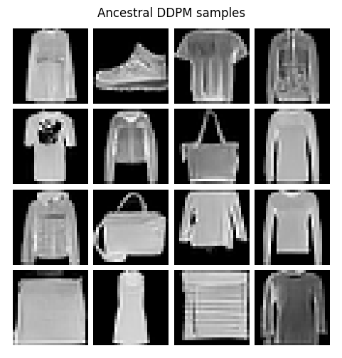
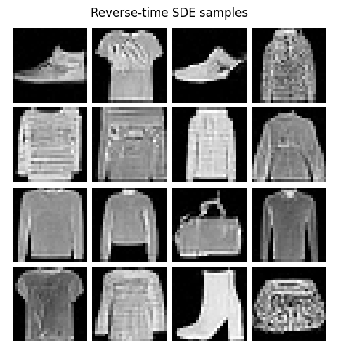
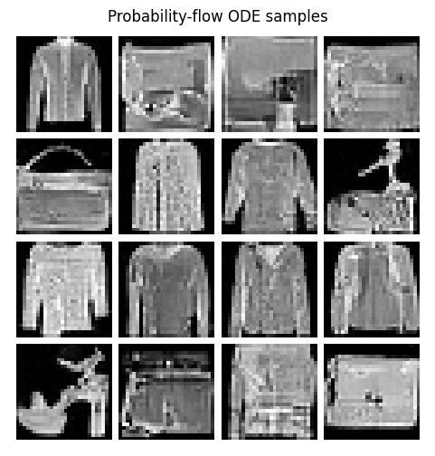
The ancestral DDPM sampler, the reverse-time SDE solver, and the probability-flow ODE solver all start from Gaussian noise and query the same network. They differ only in how they convert the score information into a trajectory.
The main numerical subtlety is that the denoiser was trained with a discrete variance schedule. To interpret that schedule in continuous time, one should remember that the discrete coefficients behave like small increments of a continuous noise rate multiplied by a timestep. Equivalently, the continuous drift and diffusion must be scaled so that one solver step over a time interval of length roughly \(1/T\) has the same magnitude as one DDPM step. With that scaling in place, the reverse-SDE and probability-flow updates become consistent with the pretrained DDPM denoiser rather than being far too weak to denoise meaningfully.
@torch.no_grad()
def sample_ddpm(model, n_samples=16, show_progress=True):
    model.eval()
    x = torch.randn(n_samples, channels, image_size, image_size, device=device)

    reverse_steps = reversed(range(timesteps))
    if show_progress:
        reverse_steps = tqdm(reverse_steps, total=timesteps, desc="ddpm sampling", leave=False)
    for t_scalar in reverse_steps:
        t = torch.full((n_samples,), t_scalar, device=device, dtype=torch.long)
        predicted_noise = model(x, t)
        beta_t = extract(betas, t, x.shape)
        sqrt_one_minus_alpha_t = extract(sqrt_one_minus_alphas, t, x.shape)
        sqrt_recip_bar_alpha_t = extract(sqrt_recip_bar_alphas, t, x.shape)
        model_mean = sqrt_recip_bar_alpha_t * (x - beta_t * predicted_noise / sqrt_one_minus_alpha_t)

        if t_scalar > 0:
            variance = extract(posterior_variance, t, x.shape)
            x = model_mean + torch.sqrt(variance) * torch.randn_like(x)
        else:
            x = model_mean

    x = x.clamp(-1, 1)
    return 0.5 * (x + 1.0)


@torch.no_grad()
def sample_reverse_sde(model, n_samples=16, num_steps=300, show_progress=True, x_init=None):
    model.eval()
    x = torch.randn(n_samples, channels, image_size, image_size, device=device) if x_init is None else x_init.clone().to(device)
    time_grid = torch.linspace(1.0, 1.0 / timesteps, num_steps, device=device)
    dt = 1.0 / num_steps

    iterator = time_grid
    if show_progress:
        iterator = tqdm(time_grid, total=num_steps, desc="reverse sde", leave=False)

    for tau in iterator:
        t_scalar = min(int(round(tau.item() * (timesteps - 1))), timesteps - 1)
        t = torch.full((n_samples,), t_scalar, device=device, dtype=torch.long)

        # Convert the discrete DDPM variance increment into a continuous-time rate.
        beta_cont = (timesteps * betas[t]).view(-1, 1, 1, 1)
        pred_noise = model(x, t)
        score = -pred_noise / extract(sqrt_one_minus_alphas, t, x.shape).clamp(min=1e-5)

        drift = -0.5 * beta_cont * x - beta_cont * score
        diffusion = torch.sqrt(beta_cont)
        x = x - drift * dt + diffusion * torch.sqrt(torch.tensor(dt, device=device)) * torch.randn_like(x)

    x = x.clamp(-1, 1)
    return 0.5 * (x + 1.0)


@torch.no_grad()
def sample_probability_flow_ode(model, n_samples=16, num_steps=300, show_progress=True, x_init=None):
    model.eval()
    x = torch.randn(n_samples, channels, image_size, image_size, device=device) if x_init is None else x_init.clone().to(device)
    time_grid = torch.linspace(1.0, 1.0 / timesteps, num_steps, device=device)
    dt = 1.0 / num_steps

    iterator = time_grid
    if show_progress:
        iterator = tqdm(time_grid, total=num_steps, desc="pf ode", leave=False)

    for tau in iterator:
        t_scalar = min(int(round(tau.item() * (timesteps - 1))), timesteps - 1)
        t = torch.full((n_samples,), t_scalar, device=device, dtype=torch.long)

        beta_cont = (timesteps * betas[t]).view(-1, 1, 1, 1)
        pred_noise = model(x, t)
        score = -pred_noise / extract(sqrt_one_minus_alphas, t, x.shape).clamp(min=1e-5)

        velocity = -0.5 * beta_cont * x - 0.5 * beta_cont * score
        x = x - velocity * dt

    x = x.clamp(-1, 1)
    return 0.5 * (x + 1.0)
Visual Comparison of DDPM, Reverse SDE, and Probability-Flow ODE#
Looking at the generated grids makes the distinction concrete. The ancestral DDPM and the reverse-time SDE both keep randomness in the trajectory. The probability-flow ODE produces a deterministic transport once the terminal Gaussian sample is fixed.
ddpm_samples = sample_ddpm(model, n_samples=16)
sde_samples = sample_reverse_sde(model, n_samples=16, num_steps=300)
pf_samples = sample_probability_flow_ode(model, n_samples=16, num_steps=300)

for title, samples in [
    ("Ancestral DDPM samples", ddpm_samples),
    ("Reverse-time SDE samples", sde_samples),
    ("Probability-flow ODE samples", pf_samples),
]:
    plt.figure(figsize=(6, 6))
    plt.imshow(utils.make_grid(samples.cpu(), nrow=4, pad_value=1.0).permute(1, 2, 0), cmap='gray')
    plt.axis('off')
    plt.title(title)
    plt.show()
Fixing the Terminal Noise#
A deterministic solver reveals itself most clearly when the starting noise is held fixed. Re-running the probability-flow ODE from the same terminal sample produces the same trajectory. Re-running the reverse-time SDE does not, because fresh Gaussian perturbations are injected during integration.
shared_noise = torch.randn(8, channels, image_size, image_size, device=device)

pf_first = sample_probability_flow_ode(model, n_samples=8, num_steps=300, x_init=shared_noise)
pf_second = sample_probability_flow_ode(model, n_samples=8, num_steps=300, x_init=shared_noise)

sde_first = sample_reverse_sde(model, n_samples=8, num_steps=300, x_init=shared_noise)
sde_second = sample_reverse_sde(model, n_samples=8, num_steps=300, x_init=shared_noise)

for title, samples in [
    ("PF-ODE from fixed terminal noise | run 1", pf_first),
    ("PF-ODE from fixed terminal noise | run 2", pf_second),
    ("Reverse SDE from fixed terminal noise | run 1", sde_first),
    ("Reverse SDE from fixed terminal noise | run 2", sde_second),
]:
    plt.figure(figsize=(10, 2.6))
    plt.imshow(utils.make_grid(samples.cpu(), nrow=8, pad_value=1.0).permute(1, 2, 0), cmap='gray')
    plt.axis('off')
    plt.title(title)
    plt.show()




Batched FID and KID Across Samplers#
Because the denoiser is fixed, the metric comparison is genuinely a comparison among samplers. The real-image statistics are accumulated once, while fake images are generated in small batches to keep memory usage controlled.
def prepare_for_metrics(images):
    if images.size(1) == 1:
        images = images.repeat(1, 3, 1, 1)
    return images.clamp(0.0, 1.0)


@torch.no_grad()
def compute_sampler_metrics(sample_fn, real_loader, num_fake=1000, metric_batch_size=64):
    fid = FrechetInceptionDistance(feature=2048, normalize=True, reset_real_features=False).to(device)
    kid = KernelInceptionDistance(subset_size=50, normalize=True, reset_real_features=False).to(device)

    real_seen = 0
    for real_images, _ in tqdm(real_loader, desc="real features", leave=False):
        real_images = real_images.to(device)
        if real_seen >= num_fake:
            break
        current = min(real_images.size(0), num_fake - real_seen)
        real_batch = prepare_for_metrics(0.5 * (real_images[:current] + 1.0))
        fid.update(real_batch, real=True)
        kid.update(real_batch, real=True)
        real_seen += current

    fake_seen = 0
    while fake_seen < num_fake:
        batch_n = min(metric_batch_size, num_fake - fake_seen)
        fake_images = sample_fn(batch_n).to(device)
        fake_batch = prepare_for_metrics(fake_images)
        fid.update(fake_batch, real=False)
        kid.update(fake_batch, real=False)
        fake_seen += batch_n

    kid_mean, kid_std = kid.compute()
    return {
        "fid": float(fid.compute().item()),
        "kid_mean": float(kid_mean.item()),
        "kid_std": float(kid_std.item()),
    }
sampler_metrics = {
    "ddpm": compute_sampler_metrics(lambda n: sample_ddpm(model, n_samples=n, show_progress=False), test_loader),
    "reverse_sde": compute_sampler_metrics(lambda n: sample_reverse_sde(model, n_samples=n, num_steps=300, show_progress=False), test_loader),
    "pf_ode": compute_sampler_metrics(lambda n: sample_probability_flow_ode(model, n_samples=n, num_steps=300, show_progress=False), test_loader),
}
sampler_metrics
c:\Users\tivog\deep-generative-models\.venv\lib\site-packages\torchmetrics\utilities\prints.py:43: UserWarning: Metric `Kernel Inception Distance` will save all extracted features in buffer. For large datasets this may lead to large memory footprint.
  warnings.warn(*args, **kwargs)
{'ddpm': {'fid': 52.791141510009766,
  'kid_mean': 0.02676919475197792,
  'kid_std': 0.00867660716176033},
 'reverse_sde': {'fid': 52.0502815246582,
  'kid_mean': 0.02173004113137722,
  'kid_std': 0.007207334972918034},
 'pf_ode': {'fid': 72.84211730957031,
  'kid_mean': 0.040892452001571655,
  'kid_std': 0.008945678360760212}}