
Random Variables, Latent Variables, and Deep Latent Variable Models#
Modern generative modeling is impossible to understand well without a comfortable command of basic probability. This chapter therefore pauses before the main model families and develops the probabilistic language that will recur everywhere: joint distributions, marginalization, conditional independence, Bayes’ theorem, and latent variable models. The aim is not to turn the course into a full probability textbook, but to make every later derivation readable and conceptually motivated.
The key modeling move is the introduction of an unobserved variable \(\boldsymbol{z}\). Instead of trying to model the full complexity of the image distribution directly in pixel space, we imagine that an image \(\boldsymbol{x}\) is generated conditionally on some hidden explanatory factors collected in \(\boldsymbol{z}\). This does not mean that the world literally contains a clean low-dimensional coordinate system for every dataset, but it captures an idea that is often fruitful in practice: images may lie near a structured set of much lower intrinsic complexity than raw ambient dimension suggests.
In terms of course flow, this is the chapter where the philosophical language of generative modeling becomes operational mathematics. The previous chapter argued that a generative model should learn the law of images rather than only a decision boundary. The present chapter now asks how such a law can be factorized, marginalized, conditioned, and inverted. By the end of it, the reader should be ready not just to admire latent-variable models intuitively, but to read their formulas without hidden gaps.
There is a pedagogical tension in probability-heavy chapters of machine-learning courses. If the discussion is too short, the later formulas look unmotivated and symbolic. If it is too abstract, students may lose sight of why these ideas matter for images. The right compromise here is to tie every definition to the latent-variable question that motivates the chapter. Why do we care about conditional distributions? Because later we shall write \(p_\theta(\boldsymbol{x} | \boldsymbol{z})\). Why do we care about marginals? Because later we shall need to integrate out \(\boldsymbol{z}\) to obtain \(p_\theta(\boldsymbol{x})\). Why do we care about Bayes’ theorem? Because later we shall need to relate the generative direction \(p(\boldsymbol{x} | \boldsymbol{z})p(\boldsymbol{z})\) to the inference direction \(p(\boldsymbol{z} | \boldsymbol{x})\).
This chapter should therefore be read less as a detached review of probability and more as the assembly of the language required by the rest of the course. The notation may be classical, but its purpose is modern: to make deep latent-variable models readable rather than magical.
Joint, Marginal, and Conditional Distributions#
Suppose \(\boldsymbol{x}\) and \(\boldsymbol{z}\) are random variables with joint density \(p(\boldsymbol{x}, \boldsymbol{z})\). From the joint object one obtains the marginal laws by integration:
When \(p(\boldsymbol{z}) > 0\), the conditional density is defined by
To make the notation concrete, let us keep one running example for this whole section. We sample one card uniformly from a standard 52-card deck. Let \(\boldsymbol{x}\) be the suit of the sampled card, so \(\boldsymbol{x} \in \{\text{hearts}, \text{diamonds}, \text{clubs}, \text{spades}\}\), and let \(\boldsymbol{z}\) be the color of the sampled card, so \(\boldsymbol{z} \in \{\text{red}, \text{black}\}\). Then \(p(\boldsymbol{x}=\text{hearts}) = 13/52 = 1/4\), \(p(\boldsymbol{z}=\text{red}) = 26/52 = 1/2\), and
The joint distribution tells us how suit and color occur together, the marginals forget one variable and keep only the law of the other, and the conditional distribution asks how the probability changes once some information is revealed.
These equations are elementary, but in generative modeling they carry enormous practical meaning. The joint density is often easier to specify than the marginal one. If we choose a prior \(p(\boldsymbol{z})\) and a conditional model \(p_\theta(\boldsymbol{x} | \boldsymbol{z})\), then the induced data density becomes
This is the canonical latent-variable construction.
Theorem 4 (Law of total probability for latent-variable models)
Let \(\boldsymbol{x}\) and \(\boldsymbol{z}\) be random variables with joint density \(p(\boldsymbol{x}, \boldsymbol{z})\). Then the marginal density of \(\boldsymbol{x}\) satisfies
Proof. Starting from the definition of conditional density,
Integrating both sides with respect to \(\boldsymbol{z}\) gives
The left-hand side is precisely the marginal density \(p(\boldsymbol{x})\), which proves the result.
In the card example, the same formula becomes
Here the first term is \((1/2)(1/2)\) because among red cards half are hearts, while the second term is \(0 \cdot (1/2)\) because no black card is a heart. So the formula gives \(p(\boldsymbol{x}=\text{hearts}) = (1/2)(1/2) + 0 \cdot (1/2) = 1/4\).
This theorem is basic probability, but it is also the exact formula that turns latent-variable modeling into a generative model for observations. The whole difficulty of models such as VAEs begins here: the formula is conceptually clean, but the integral is usually intractable once the conditional model is implemented by a flexible neural network.
Theorem 5 (Bayes’ theorem)
If \(p(\boldsymbol{x}) > 0\), then
Proof. By the definition of conditional density,
Equating the two expressions and dividing by \(p(\boldsymbol{x})\) gives the result.
Bayes’ theorem is the algebraic bridge between generation and inference. The factorization \(p(\boldsymbol{x} | \boldsymbol{z}) p(\boldsymbol{z})\) describes how data arise from latent causes. The posterior \(p(\boldsymbol{z} | \boldsymbol{x})\) describes what can be inferred about those causes once an image has been observed. A large part of modern generative modeling consists of dealing with the fact that the posterior is informative and useful, but often hard to compute exactly.
In the card example, Bayes’ theorem lets us reverse the direction of reasoning. If we know the card is red, then the probability of hearts is \(p(\boldsymbol{x}=\text{hearts} \mid \boldsymbol{z}=\text{red}) = 1/2\). Bayes tells us how to invert this and ask for the probability that the card is red once we know that it is a heart:
That answer is obvious once one thinks about the deck, because every heart is red. But the formula matters because it teaches the pattern: one direction of conditioning may be easy to describe, while the reverse direction must be computed. In short, Bayes’ theorem tells us how to convert a forward description such as “given the color, what is the suit” into a backward description such as “given the suit, what is the color.”
It is worth stressing what Bayes’ theorem means operationally. In the generative direction we imagine that hidden causes are sampled first and images appear afterward. In the inferential direction we observe the image and try to reason backward about which hidden causes might have produced it. These two viewpoints are mathematically equivalent because they describe the same joint distribution, but computationally they can be very different. Sampling from the prior and then from the decoder may be easy, while computing the exact posterior may be hard. This asymmetry is one of the defining features of modern deep latent-variable models.
The card example is deliberately simple, but it already shows the asymmetry clearly. In a real generative model, this same asymmetry appears again in a much richer form: the forward direction defines how hidden causes generate visible data, while the backward direction asks which hidden causes best explain what we observed.
A simple image example makes the same point in the setting we actually care about. Imagine that \(\boldsymbol{z}\) stores two hidden factors: digit identity and stroke thickness. The decoder answers the forward question: if the hidden factors correspond to “3” with thick strokes, what image is likely to appear. The posterior answers the reverse question: after seeing a specific handwritten image, which hidden identities and stroke styles are plausible explanations.
For intuition, one may think even more broadly of a portrait image. The latent variable might encode identity, pose, lighting, hairstyle, or other hidden factors. The conditional model answers the question: if these hidden factors were given, what image would likely be produced. The posterior answers the reverse question: given this observed image, which hidden factors are plausible. Later, the VAE will formalize exactly how to deal with the fact that the reverse question is difficult.
Conditional Independence and Graphical Structure#
Conditional independence statements are a compact way to encode modeling assumptions. For three random variables \(\boldsymbol{x}\), \(\boldsymbol{y}\), and \(\boldsymbol{z}\), the notation \(\boldsymbol{x} \perp \boldsymbol{y} | \boldsymbol{z}\) means that once \(\boldsymbol{z}\) is known, additional knowledge of \(\boldsymbol{y}\) provides no further information about \(\boldsymbol{x}\). In density form, this becomes
Probabilistic graphical models visualize these assumptions and guide factorization choices. In the simplest latent-variable graph \(\boldsymbol{z} \to \boldsymbol{x}\), the prior on \(\boldsymbol{z}\) and the conditional model of \(\boldsymbol{x}\) given \(\boldsymbol{z}\) fully determine the joint law.
For intuition, one may think of \(\boldsymbol{z}\) as encoding coarse semantic information such as pose, object identity, lighting, or style, and of \(\boldsymbol{x}\) as the final image produced from those factors. This interpretation is never exact, but it is helpful. It explains why latent representations are appealing: they may provide a more manageable coordinate system in which the complexity of the data is disentangled or at least organized.
A common source of confusion is that graphical models look discrete and symbolic while neural generative models look continuous and high-dimensional. In reality, they are describing complementary aspects of the same model. The graph expresses the dependency structure. The neural network expresses the functional form of a conditional distribution. One should therefore not think of probabilistic graphical models as obsolete toys that were replaced by deep learning. They remain one of the clearest ways to understand what is assumed to depend on what.
This point matters for model criticism as well. If a generative model fails, the failure may come from many sources: the decoder may be too weak, the optimization may be poor, the latent prior may be badly chosen, or the dependency structure itself may be too naive. Graphical intuition helps us separate these possibilities conceptually.
The Manifold Hypothesis as a Modeling Heuristic#
The manifold hypothesis informally states that high-dimensional data encountered in practice often concentrate near a set of much lower intrinsic dimension. For images, this means that although a vectorized image may live in \(\mathbb{R}^d\) with enormous \(d\), only a small subset of configurations correspond to meaningful natural images. Most points in ambient space look like noise. Generative modeling can therefore be interpreted as the attempt to learn the geometry and probability structure of this thin, complicated subset.
It is important not to overstate the hypothesis. The data need not lie on a perfectly smooth manifold, and realistic datasets are usually noisy, multimodal, and heterogeneous. Still, the heuristic remains useful because it motivates latent variables. If images are controlled by a smaller collection of underlying factors, a latent-variable model may capture them more effectively than a direct unstructured density in pixel space.
The manifold hypothesis should be understood as a modeling suggestion, not as dogma. It tells us that high-dimensional data are often structured enough that a lower-dimensional description is meaningful. It does not tell us what the right dimension is, whether the structure is globally smooth, or whether one latent variable is enough. In practice, this is why modern latent-variable models often use moderately large latent spaces, hierarchical latent structures, or richly structured decoders. The hypothesis justifies the search for hidden explanatory coordinates; it does not remove the need for careful model design.
Deep Latent Variable Models#
A deep latent variable model combines the probabilistic construction of latent variables with the expressive power of neural networks. The generic factorization is
where \(p(\boldsymbol{z})\) is often chosen to be a simple standard Gaussian and the conditional density \(p_\theta(\boldsymbol{x} | \boldsymbol{z})\) is parameterized by a decoder network.
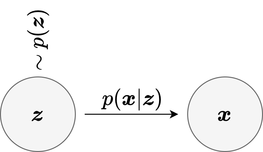
Fig. 11 The basic deep latent-variable factorization: first sample a latent variable \(\boldsymbol{z}\) from a simple prior, then generate the observation through the conditional law \(p_\theta(\boldsymbol{x} | \boldsymbol{z})\).#
This picture is worth placing early because it explains the key probabilistic move immediately. Instead of trying to model \(p_{gt}(\boldsymbol{x})\) in one shot, we enlarge the model by introducing a hidden variable and writing a joint law \(p_\theta(\boldsymbol{x}, \boldsymbol{z})\). The joint object factorizes naturally into a prior over hidden causes and a conditional decoder that explains how those causes produce visible data.
The real hope behind this construction is that the conditional distribution \(p_{gt}(\boldsymbol{x} | \boldsymbol{z})\) may be much simpler than the full marginal distribution \(p_{gt}(\boldsymbol{x})\). If \(\boldsymbol{z}\) captures the main explanatory factors of variation, then once \(\boldsymbol{z}\) is fixed, much of the ambiguity in the image is gone. Modeling one narrow conditional family can therefore be easier than modeling the full multimodal data distribution directly.
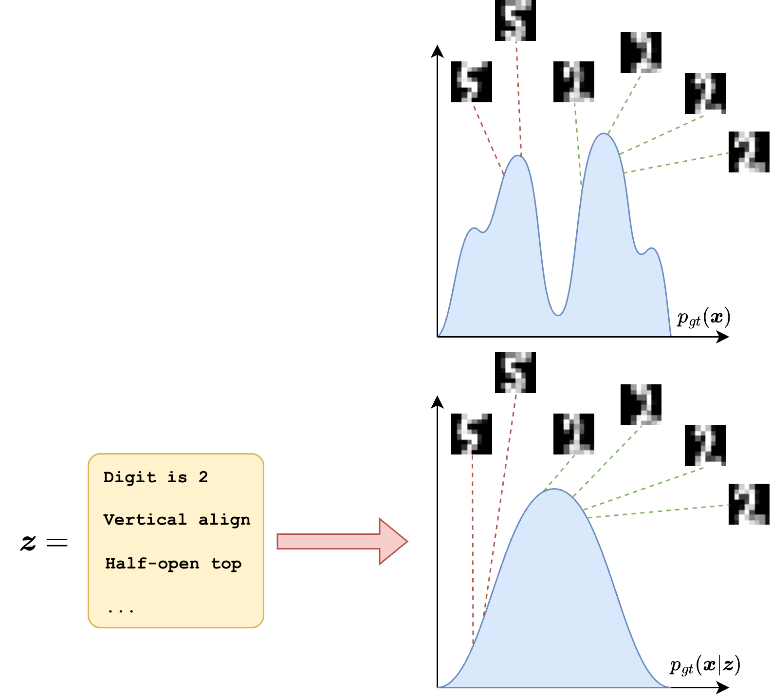
Fig. 12 A latent variable can simplify the modeling task dramatically: the full data distribution \(p_{gt}(\boldsymbol{x})\) may be highly complex, while the conditional distribution \(p_{gt}(\boldsymbol{x} | \boldsymbol{z})\) becomes much more structured once the latent description is known.#
Learning requires the marginal likelihood
while inference requires the posterior \(p_\theta(\boldsymbol{z} | \boldsymbol{x})\). These two objects are exactly where the main difficulty lies. The model is expressive because the decoder is a neural network, but that same flexibility generally destroys analytic tractability. So the latent variable simplifies the conceptual structure of the distribution, but it also introduces the computational challenge of marginalization and posterior inference.
Numerical Example: A Handwritten Digit as \((\boldsymbol{x}, \boldsymbol{z})\)
Let \(\boldsymbol{x}\) be the image of a handwritten digit “2”. The corresponding latent variable \(\boldsymbol{z}\) is not another image, but a hidden description of that drawing. One coordinate of \(\boldsymbol{z}\) might encode digit identity, another stroke thickness, another slant, and another whether the bottom loop is open or closed.
In a generative story, we might first sample a latent description such as \(\boldsymbol{z} = (\text{digit}=2,\ \text{thickness}=0.7,\ \text{slant}=-0.2,\ \text{curvature}=0.9)\) and then draw the image from \(p_\theta(\boldsymbol{x} | \boldsymbol{z})\). In the inferential story, we observe the actual pixels of a handwritten “2” and ask which hidden descriptions are plausible. The posterior \(p_\theta(\boldsymbol{z} | \boldsymbol{x})\) should place high probability on descriptions compatible with a “2” and very low probability on descriptions corresponding to a “7” or to extreme stroke styles not present in the image.
This example is intentionally informal, but it captures the main idea: \(\boldsymbol{x}\) is the visible object, while \(\boldsymbol{z}\) is a compressed hidden explanation of why that object looks the way it does.
The variational autoencoder can now be seen as a disciplined answer to this difficulty. Instead of computing the posterior exactly, it introduces an approximating family \(q_\phi(\boldsymbol{z} | \boldsymbol{x})\) and optimizes a lower bound to the log-likelihood. This is the first major point where neural networks, probability, and optimization fully meet. Background material for this probabilistic viewpoint may be found in [Bis06], while the deep latent-variable perspective is developed in [KW13] and [RMW14].