
Variational Autoencoders: ELBO, Inference, and Learning#
Generative modeling can be formulated as a maximum likelihood problem. We observe samples \(\boldsymbol{x}_1,\ldots,\boldsymbol{x}_n\) from an unknown data distribution \(p_{gt}(\boldsymbol{x})\), and we introduce a parametric model \(p_\theta(\boldsymbol{x})\) that should assign high probability to images that could plausibly come from that distribution. In population form, the ideal objective is
and in finite data form this becomes the empirical log-likelihood
The deep latent-variable view developed earlier gives a structured way to define \(p_\theta(\boldsymbol{x})\). An image is assumed to be generated from hidden factors \(\boldsymbol{z}\), such as shape, pose, thickness, or style. The joint model is \(p_\theta(\boldsymbol{x},\boldsymbol{z}) = p_\theta(\boldsymbol{x}|\boldsymbol{z})p(\boldsymbol{z})\), so generation has two steps: sample \(\boldsymbol{z}\) from a prior, then sample or decode \(\boldsymbol{x}\) from \(p_\theta(\boldsymbol{x}|\boldsymbol{z})\). The marginal likelihood required by maximum likelihood is therefore
The usual prior choice is \(p(\boldsymbol{z}) = \mathcal{N}(\boldsymbol{0},\boldsymbol{I})\).
This Gaussian prior is a modeling assumption. It gives a simple latent reference distribution that is easy to sample, has a smooth geometry, and leads to analytic KL terms. The assumption is useful because the decoder is nonlinear: a neural network can transform a simple latent distribution into a complicated image distribution. The cost of this simplicity is that the model must learn a latent organization compatible with the standard Gaussian prior.
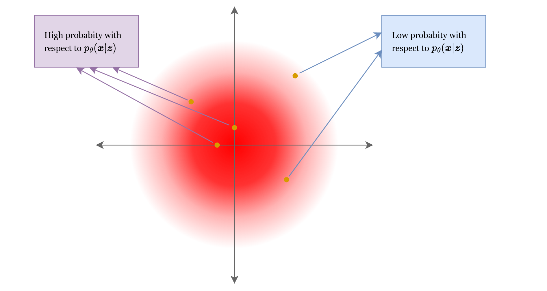
Fig. 13 Not all the samples \(\boldsymbol{z} \sim p(\boldsymbol{z})\) are equally relevant for \(p_\theta(\boldsymbol{x} | \boldsymbol{z})\).#
The difficulty appears immediately. The integral defining \(p_\theta(\boldsymbol{x})\) is usually intractable. The latent variable may be high-dimensional, and the decoder is a neural network, so the integral has no closed form. Direct maximum likelihood is therefore blocked.
A natural idea is to focus on the latent values that matter for the observed image. If \(\boldsymbol{x}\) is a boot, not every \(\boldsymbol{z}\) is equally relevant. Some latent configurations should explain that image much better than others. This suggests looking at the posterior distribution over latent variables:
This posterior is exactly the distribution one would like to use for inference. It tells us which latent explanations are plausible after seeing the image. Unfortunately, Bayes’ theorem has not removed the problem. The denominator is the same intractable marginal likelihood. The posterior is therefore intractable for the same reason the likelihood is intractable.
The variational idea is to introduce a new distribution \(q_\phi(\boldsymbol{z}|\boldsymbol{x})\), chosen from a tractable family and implemented by a neural network. Its role is to approximate the true posterior \(p_\theta(\boldsymbol{z}|\boldsymbol{x})\). This is the recognition model, or encoder. The word variational means that exact inference is replaced by optimization over an approximate family. The VAE is built from this compromise: the decoder defines the generative model, while the encoder makes approximate posterior inference fast enough to train the model.
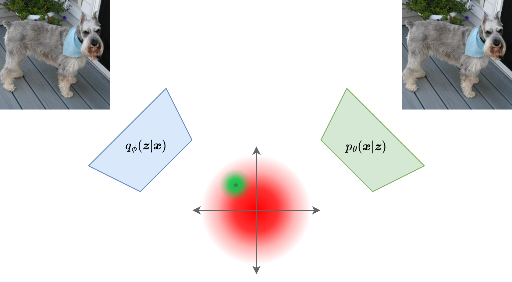
Fig. 14 The autoencoder-like structure of VAE.#
Derivation of the Evidence Lower Bound#
Start from the log-likelihood of one observation. For any tractable density \(q_\phi(\boldsymbol{z}|\boldsymbol{x})\) whose support covers the relevant latent region, write
This identity only multiplies and divides by the approximate posterior. It does not approximate anything yet. The approximation enters when Jensen’s inequality is applied to move the logarithm inside the expectation.
Theorem 6 (Evidence lower bound)
For any density \(q_\phi(\boldsymbol{z}|\boldsymbol{x})\) whose support contains the relevant support of \(p_\theta(\boldsymbol{x},\boldsymbol{z})\),
The right-hand side is called the evidence lower bound, or ELBO.
Proof. Write the marginal likelihood as an expectation under \(q_\phi(\boldsymbol{z}|\boldsymbol{x})\):
Since \(\log\) is concave, Jensen’s inequality gives
Expanding the logarithm gives the stated expression.
The gap introduced by Jensen’s inequality is the price paid for replacing exact marginalization with tractable posterior sampling. If \(q_\phi(\boldsymbol{z}|\boldsymbol{x})\) matches the true posterior, the bound becomes tight. If it is a poor approximation, the bound may be loose even when the decoder is expressive.
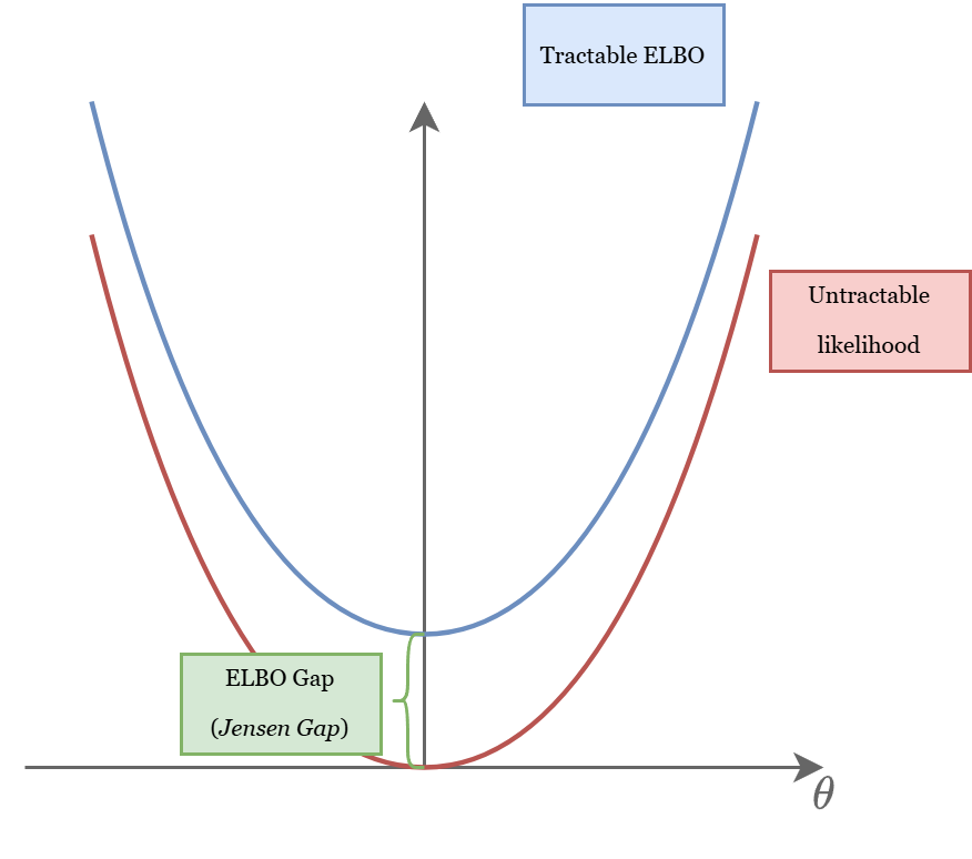
Fig. 15 Minimizing ELBO implicity optimizes the negative log-likelihood.#
The ELBO becomes more interpretable after expanding the joint density:
This is the key moment where the VAE begins to look like an autoencoder. The first term asks the decoder to reconstruct or explain \(\boldsymbol{x}\) from latent samples produced by the encoder. If the observation model is Bernoulli, this term becomes a binary cross-entropy reconstruction criterion. If the observation model is Gaussian with fixed variance, it becomes proportional to a squared-error reconstruction criterion:
Theorem 7 (VAE as regularized autoencoder)
Assuming \(p_\theta(\boldsymbol{x} | \boldsymbol{z}) = \mathcal{N}(\mu_\theta(\boldsymbol{z}), \sigma^2 \boldsymbol{I})\), where \(\mu_\theta(\boldsymbol{z})\) is a neural network, then:
is a Mean Squared Error (MSE) term between the output \(\mu_\theta(\boldsymbol{z})\) of the neural network, and the true image \(\boldsymbol{x}\).
Proof. Recall that \(\mathcal{N}(\mu_\theta(\boldsymbol{z}), \sigma^2 \boldsymbol{I})\) corresponds to:
Therefore:
Removing the terms that does not depend on \(\theta\) (whose gradient is zero), it we obtain \(\log p_\theta(\boldsymbol{z} | \boldsymbol{x}) \propto - \frac{ \left\| \boldsymbol{x} - \mu_\theta(\boldsymbol{z}) \right\|^2}{2\sigma^2}\), which is precisely the MSE between \(\boldsymbol{x}\) and \(\mu_\theta(\boldsymbol{z})\).
The second term is the regularizer. It compares the encoder distribution for this image with the prior distribution used for generation. Without this term, the encoder could place each training image in arbitrary isolated regions of latent space, producing a deterministic autoencoder that reconstructs well but cannot be sampled reliably. With the KL term, the encoded distributions are encouraged to live near a common reference geometry. This is why sampling from \(p(\boldsymbol{z})\) after training has a chance to produce meaningful images.
In loss-minimization form, one minimizes the negative ELBO:
This is the reconstruction-plus-regularization form used in implementation.
Reading the ELBO
The ELBO has two simultaneous roles. It is a tractable lower bound on the intractable log-likelihood, and it is the objective that gives the VAE its autoencoder-like form: a reconstruction term plus a KL regularization term.
Theorem 8 (ELBO decomposition with posterior gap)
For every observation \(\boldsymbol{x}\),
Proof. Starting from the ELBO expression,
Add and subtract \(\log p_\theta(\boldsymbol{z} | \boldsymbol{x})\). Using
we obtain
The expectation is exactly the Kullback-Leibler divergence between the approximate and exact posterior, which proves the identity.
The identity explains why the bound is useful. Maximizing the ELBO pushes upward the data log-likelihood while pushing downward the gap between the recognition model and the true posterior. The quality of generation and the quality of inference are therefore coupled. If the approximate posterior family is too restrictive, the learned decoder may adapt to what the encoder can represent rather than to the best possible latent-variable explanation of the data.
The same identity also explains why the ELBO can be viewed as a controlled approximation to maximum likelihood. The real target is still \(\log p_\theta(\boldsymbol{x})\). The ELBO is used because it is tractable, differentiable, and expresses the two operations the model must learn: reconstruct from likely latent explanations and keep those explanations compatible with the prior.
Numerical Example: Reading the ELBO Terms
Suppose an encoder sees an image of a sneaker and outputs a two-dimensional Gaussian posterior with mean \(\boldsymbol{\mu} = (1.2, -0.4)\) and standard deviations \((0.5, 0.8)\). The corresponding variational distribution says that the image is encoded near the point \((1.2, -0.4)\) in latent space, but with noticeable uncertainty, especially in the second coordinate.
If the decoder reconstructs the sneaker well, the reconstruction term in the ELBO is favorable. But the KL term also checks how far this posterior has drifted from the standard Gaussian prior. Here the first coordinate is shifted away from zero, so there is a regularization cost. The ELBO is therefore balancing two pressures at once: keep enough latent information to reconstruct the sneaker, but do not let the posterior wander arbitrarily far from the simple prior that we want to sample from at generation time.
The encoder \(q_\phi(\boldsymbol{z}|\boldsymbol{x})\) is often called an amortized inference model because a single neural network is trained to solve approximate inference for every observation. Instead of optimizing a separate variational distribution from scratch for each image, the encoder learns a direct map from images to posterior parameters. This is computationally powerful, but it introduces another approximation layer. The encoder may fail to represent the true posterior because the chosen family is too simple, because the neural network is not expressive enough, or because one shared inference model cannot serve all observations equally well.
This perspective is useful when reading VAE variants. Some variants enrich the variational family, some redesign the decoder likelihood, some modify the KL weight, some learn a richer prior, and some reduce amortization error. The classical ELBO is therefore the organizing baseline, not the final word.
From Latent-Variable Modeling to a Stochastic Autoencoder#
The ELBO gives the VAE its familiar architecture. The approximate posterior \(q_\phi(\boldsymbol{z}|\boldsymbol{x})\) is represented by an encoder network. The likelihood model \(p_\theta(\boldsymbol{x}|\boldsymbol{z})\) is represented by a decoder network. Between them sits a stochastic latent variable sampled from the encoder distribution.
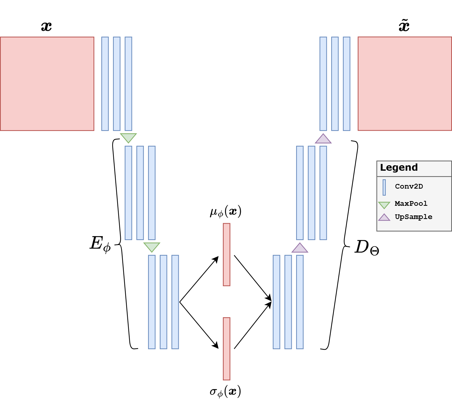
Fig. 16 A convolutional variational autoencoder. The encoder maps an image to the parameters of a latent Gaussian, the stochastic bottleneck samples a code, and the decoder maps that code back into image logits.#
The encoder maps an image to the parameters of a distribution over latent explanations. The stochastic bottleneck draws a latent code from that distribution. The decoder maps the sampled code to the parameters of the observation model. This creates an autoencoder-like computation, but the latent code is probabilistic and the encoded distributions are regularized toward the prior used for generation.
In this sense, a VAE is a stochastic autoencoder with a probabilistic interpretation. The reconstruction path comes from the likelihood term in the ELBO. The latent-space regularization comes from the KL term. The architecture is the neural-network realization of these two terms.
Gaussian Encoders and the Reparameterization Trick#
A common VAE choice is a diagonal Gaussian encoder:
The encoder network outputs the mean vector \(\boldsymbol{\mu}_\phi(\boldsymbol{x})\) and the log-variance vector \(\log \boldsymbol{\sigma}_\phi^2(\boldsymbol{x})\). The prior is usually the standard Gaussian. With these choices, the KL term has a closed form (as we will see later), so the only stochastic part left in the objective is the reconstruction expectation.
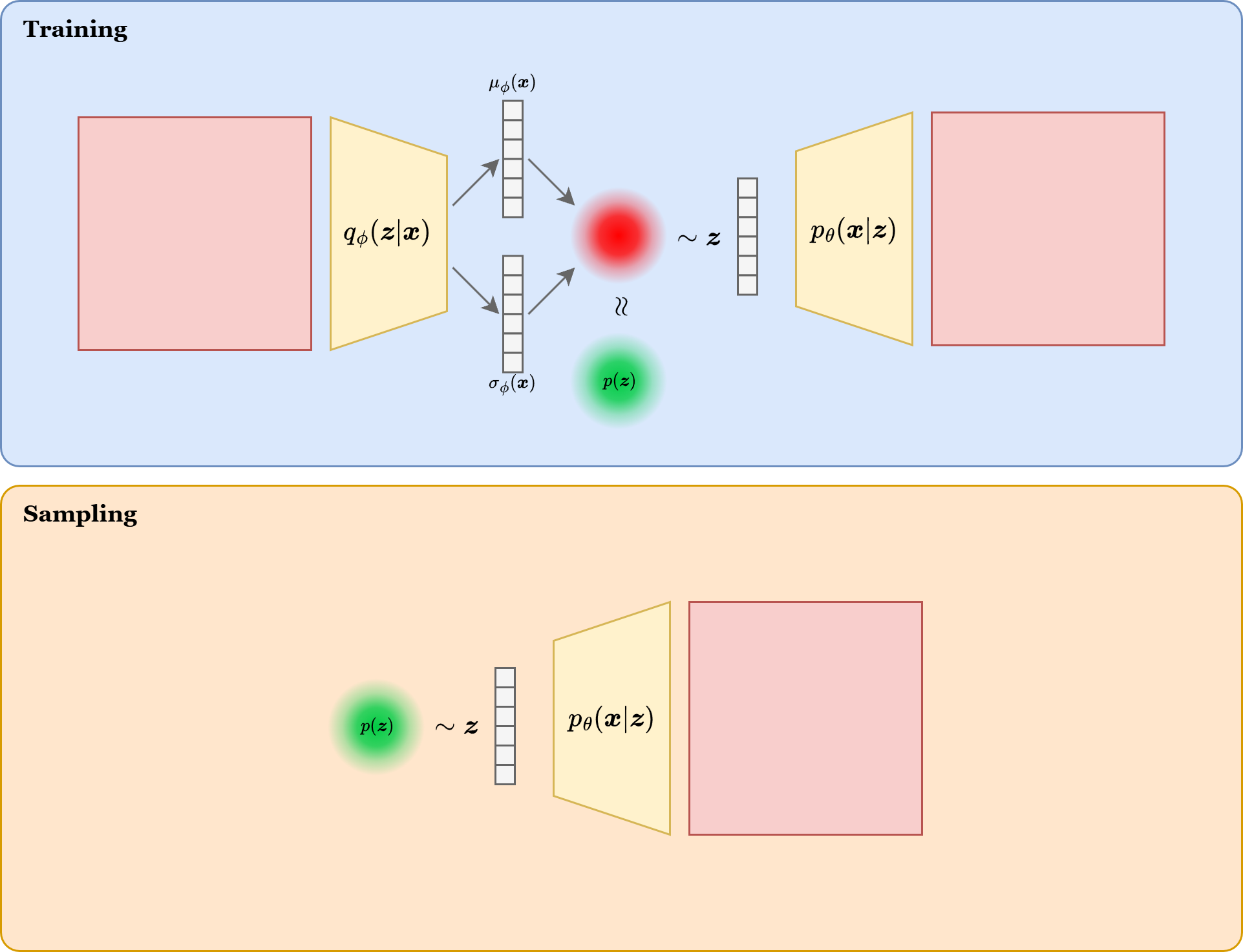
Fig. 17 Training and sampling in typical VAE setting.#
The remaining training obstacle is differentiating through a sample from \(q_\phi(\boldsymbol{z}|\boldsymbol{x})\). A sample depends on the encoder parameters, and naive sampling is not a differentiable operation with respect to those parameters. The reparameterization trick rewrites the random draw as
Now the randomness is isolated in \(\boldsymbol{\varepsilon}\), which does not depend on \(\phi\). The path from \(\boldsymbol{\mu}_\phi\), \(\boldsymbol{\sigma}_\phi\), and the decoder output remains differentiable. This is what makes standard backpropagation applicable to the ELBO.
Theorem 9 (Closed-form KL for a diagonal Gaussian encoder)
Let
and let the prior be
Then
Proof. By definition,
For the diagonal Gaussian posterior,
while for the standard Gaussian prior,
Subtracting and taking expectation under \(q\), we use
The constant \(\log(2\pi)\) terms cancel, leaving
which proves the formula.
This explicit KL formula is one of the practical reasons the Gaussian VAE became a standard baseline. The reconstruction term can be estimated with a small number of latent samples, often just one, and the regularization term is analytic. The whole objective is therefore differentiable and cheap to evaluate.
Guided Implementation#
The implementation mirrors the probabilistic notation. The encoder represents \(q_\phi(\boldsymbol{z}|\boldsymbol{x})\). Its two outputs are \(\boldsymbol{\mu}_\phi(\boldsymbol{x})\) and \(\log \boldsymbol{\sigma}_\phi^2(\boldsymbol{x})\). The reparameterization step samples \(\boldsymbol{z}\). The decoder represents \(p_\theta(\boldsymbol{x}|\boldsymbol{z})\). The loss combines the reconstruction term and the Gaussian KL term from the ELBO.
FashionMNIST is small enough to train quickly but diverse enough to make the main tradeoffs visible. Even at this scale one can see blurry reconstructions, latent regularization, posterior collapse, and the effect of changing the KL pressure.
Gaussian VAE in one line
The encoder outputs \(\boldsymbol{\mu}_\phi(\boldsymbol{x})\) and \(\log \boldsymbol{\sigma}_\phi^2(\boldsymbol{x})\), the reparameterization trick samples \(\boldsymbol{z}\) differentiably, and the decoder maps \(\boldsymbol{z}\) to the parameters of \(p_\theta(\boldsymbol{x}|\boldsymbol{z})\).
import torch
import torch.nn as nn
import torch.nn.functional as F
from pathlib import Path
from torch.utils.data import DataLoader
from torchmetrics.image.fid import FrechetInceptionDistance
from torchmetrics.image.kid import KernelInceptionDistance
from torchvision import datasets, transforms, utils
from tqdm.auto import tqdm
import matplotlib.pyplot as plt

device = torch.device("cuda" if torch.cuda.is_available() else "cpu")
torch.manual_seed(7)
if device.type == "cuda":
    torch.cuda.manual_seed_all(7)
num_workers =  0
project_root = Path.cwd() if (Path.cwd() / "_config.yml").exists() else Path.cwd().parent
DATA_ROOT = project_root / "data"

# Settings
batch_size = 128
latent_dim = 32
base_channels = 32
lr = 2e-4
epochs = 60

transform = transforms.ToTensor()

train_dataset = datasets.FashionMNIST(
    root=DATA_ROOT,
    train=True,
    download=True,
    transform=transform,
)

test_dataset = datasets.FashionMNIST(
    root=DATA_ROOT,
    train=False,
    download=True,
    transform=transform,
)

train_loader = DataLoader(
    train_dataset,
    batch_size=batch_size,
    shuffle=True,
    num_workers=num_workers,
    pin_memory=(device.type == "cuda"),
)
test_loader = DataLoader(
    test_dataset,
    batch_size=batch_size,
    shuffle=False,
    num_workers=num_workers,
    pin_memory=(device.type == "cuda"),
)
The hyperparameters deserve interpretation because they encode the assumptions of the probabilistic model. The latent dimension is the size of the information channel. If it is too small, reconstructions lose important factors. If it is too large, the model may waste capacity or make the KL term harder to interpret. The decoder capacity controls how much structure can be produced from \(\boldsymbol{z}\). A very powerful decoder may learn to model local image statistics while ignoring the latent code, whereas a weak decoder may force too much burden onto the latent representation.
The training budget is large enough to let the ELBO terms settle into a meaningful regime. A VAE trained for only a few epochs often demonstrates the code path rather than the model. The goal is to see reconstructions, samples, KL behavior, and interpolation geometry together.
class VAE(nn.Module):
    def __init__(self, latent_dim=32, base_channels=32):
        super().__init__()
        # 28x28 -> 14x14 -> 7x7.
        self.encoder = nn.Sequential(
            nn.Conv2d(1, base_channels, kernel_size=4, stride=2, padding=1),
            nn.BatchNorm2d(base_channels),
            nn.SiLU(),
            nn.Conv2d(base_channels, base_channels * 2, kernel_size=4, stride=2, padding=1),
            nn.BatchNorm2d(base_channels * 2),
            nn.SiLU(),
            nn.Conv2d(base_channels * 2, base_channels * 4, kernel_size=3, padding=1),
            nn.BatchNorm2d(base_channels * 4),
            nn.SiLU(),
            nn.Flatten(),
        )
        encoded_dim = base_channels * 4 * 7 * 7
        self.mu_head = nn.Linear(encoded_dim, latent_dim)
        self.logvar_head = nn.Linear(encoded_dim, latent_dim)

        self.decoder = nn.Sequential(
            nn.Linear(latent_dim, encoded_dim),
            nn.SiLU(),
            nn.Unflatten(1, (base_channels * 4, 7, 7)),
            nn.ConvTranspose2d(base_channels * 4, base_channels * 2, kernel_size=4, stride=2, padding=1),
            nn.BatchNorm2d(base_channels * 2),
            nn.SiLU(),
            nn.ConvTranspose2d(base_channels * 2, base_channels, kernel_size=4, stride=2, padding=1),
            nn.BatchNorm2d(base_channels),
            nn.SiLU(),
            nn.Conv2d(base_channels, 1, kernel_size=3, padding=1),
        )

    def encode(self, x):
        h = self.encoder(x)
        mu = self.mu_head(h)
        logvar = self.logvar_head(h)
        return mu, logvar

    def reparameterize(self, mu, logvar):
        # Sample through parameter-free noise so gradients can flow to mu/logvar.
        std = torch.exp(0.5 * logvar)
        eps = torch.randn_like(std)
        return mu + std * eps

    def decode(self, z):
        logits = self.decoder(z)
        return logits

    def forward(self, x):
        mu, logvar = self.encode(x)
        z = self.reparameterize(mu, logvar)
        logits = self.decode(z)
        return logits, mu, logvar


model = VAE(latent_dim=latent_dim, base_channels=base_channels).to(device)
optimizer = torch.optim.Adam(model.parameters(), lr=lr)
The method reparameterize is the code-level manifestation of the identity
This rewrite is essential for gradient-based learning. A direct sample from a parameterized Gaussian would obstruct backpropagation through the stochastic node. After reparameterization, the random source is independent of the learnable parameters, so the computational graph remains differentiable with respect to \(\phi\).
ELBO Loss in Code#
We now implement the negative ELBO. The reconstruction term is approximated by a binary cross-entropy between the reconstructed image probabilities and the input image. This corresponds to choosing a Bernoulli observation model for pixels. The KL term is the closed-form divergence between a diagonal Gaussian posterior and the standard Gaussian prior. Since optimizers minimize rather than maximize, we return the negative ELBO.
def elbo_loss(x, logits, mu, logvar):
    # Bernoulli reconstruction term for pixels in [0, 1].
    reconstruction = F.binary_cross_entropy_with_logits(
        logits,
        x,
        reduction="sum",
    )
    # Closed-form KL for a diagonal Gaussian encoder against N(0, I).
    kl = -0.5 * torch.sum(1 + logvar - mu.pow(2) - logvar.exp())
    loss = reconstruction + kl
    return loss, reconstruction, kl
A subtle implementation detail is the use of logits instead of post-sigmoid probabilities inside binary_cross_entropy_with_logits. This is the stable way to compute the Bernoulli negative log-likelihood. Conceptually, the decoder defines independent Bernoulli probabilities for pixels after a sigmoid transformation. Numerically, the loss is evaluated directly from logits to avoid instability when probabilities are close to zero or one.
The KL term in the code is exactly the closed-form diagonal Gaussian KL derived above. It is averaged over the batch so that the reconstruction and regularization terms have comparable scale in the printed diagnostics.
A second important design choice is the reconstruction law. The decoder outputs logits and the loss uses a Bernoulli-style binary cross-entropy. For grayscale images scaled to \([0,1]\), this is a simple and coherent observation model. It is not the only possible choice, and it is part of why simple VAEs often look softer than GANs or diffusion models. Pixelwise likelihoods reward the model for being locally correct, not necessarily perceptually sharp.
Training Dynamics and the Meaning of the KL Weight#
Even when one writes down the vanilla ELBO, the effective weight of the KL term is one of the most important practical quantities in the model. If the KL pressure is too strong too early, the encoder may learn to communicate too little and the latent variable becomes uninformative. If the KL pressure is too weak, reconstructions may look excellent while samples from the prior become poor because the encoded latent space drifts too far from the distribution used at generation time.
This is why the split between reconstruction and KL should be monitored during training. Those two numbers are not decorative logging. They tell us whether the latent channel is being used, whether regularization is dominating, and whether the model has found a healthy compromise.
def train_epoch(model, loader, optimizer, device):
    model.train()
    total_loss = 0.0
    total_reconstruction = 0.0
    total_kl = 0.0

    for x, _ in tqdm(loader, desc="train", leave=False):
        x = x.to(device)

        optimizer.zero_grad()
        logits, mu, logvar = model(x)
        loss, reconstruction, kl = elbo_loss(x, logits, mu, logvar)
        loss.backward()
        optimizer.step()

        total_loss += loss.item()
        total_reconstruction += reconstruction.item()
        total_kl += kl.item()

    n = len(loader.dataset)
    return {
        "loss": total_loss / n,
        "reconstruction": total_reconstruction / n,
        "kl": total_kl / n,
    }


@torch.no_grad()
def evaluate(model, loader, device):
    model.eval()
    total_loss = 0.0
    total_reconstruction = 0.0
    total_kl = 0.0

    for x, _ in tqdm(loader, desc="eval", leave=False):
        x = x.to(device)
        logits, mu, logvar = model(x)
        loss, reconstruction, kl = elbo_loss(x, logits, mu, logvar)

        total_loss += loss.item()
        total_reconstruction += reconstruction.item()
        total_kl += kl.item()

    n = len(loader.dataset)
    return {
        "loss": total_loss / n,
        "reconstruction": total_reconstruction / n,
        "kl": total_kl / n,
    }
history = {"train_loss": [], "train_kl": [], "val_loss": [], "val_kl": []}

for epoch in tqdm(range(epochs), desc="VAE epochs"):
    train_stats = train_epoch(model, train_loader, optimizer, device)
    val_stats = evaluate(model, test_loader, device)

    history["train_loss"].append(train_stats["loss"])
    history["train_kl"].append(train_stats["kl"])
    history["val_loss"].append(val_stats["loss"])
    history["val_kl"].append(val_stats["kl"])

    print(
        f"Epoch {epoch + 1:02d} | "
        f"train loss: {train_stats['loss']:.4f} | "
        f"train KL: {train_stats['kl']:.4f} | "
        f"val loss: {val_stats['loss']:.4f} | "
        f"val KL: {val_stats['kl']:.4f}"
    )
Epoch 01 | train loss: 292.7335 | train KL: 19.1436 | val loss: 260.1806 | val KL: 20.1409
Epoch 02 | train loss: 254.7370 | train KL: 19.6022 | val loss: 253.3469 | val KL: 19.5857
Epoch 03 | train loss: 250.1020 | train KL: 19.3058 | val loss: 250.3804 | val KL: 19.5410
Epoch 04 | train loss: 247.7569 | train KL: 19.0762 | val loss: 248.1927 | val KL: 18.6147
Epoch 05 | train loss: 246.3201 | train KL: 18.9794 | val loss: 248.3276 | val KL: 19.6058
Epoch 06 | train loss: 245.1999 | train KL: 18.8188 | val loss: 246.2563 | val KL: 19.0079
Epoch 07 | train loss: 244.3586 | train KL: 18.6993 | val loss: 245.7819 | val KL: 18.4176
Epoch 08 | train loss: 243.7890 | train KL: 18.6879 | val loss: 245.1527 | val KL: 18.4556
Epoch 09 | train loss: 243.1169 | train KL: 18.5695 | val loss: 244.9765 | val KL: 18.6641
Epoch 10 | train loss: 242.6527 | train KL: 18.5202 | val loss: 244.2759 | val KL: 18.4843
Epoch 11 | train loss: 242.2205 | train KL: 18.4364 | val loss: 244.0456 | val KL: 18.2308
Epoch 12 | train loss: 241.9455 | train KL: 18.4553 | val loss: 243.9405 | val KL: 18.5218
Epoch 13 | train loss: 241.5166 | train KL: 18.3376 | val loss: 243.8370 | val KL: 18.5269
Epoch 14 | train loss: 241.1947 | train KL: 18.3105 | val loss: 243.0484 | val KL: 18.9893
Epoch 15 | train loss: 240.9180 | train KL: 18.2768 | val loss: 242.8338 | val KL: 18.0846
Epoch 16 | train loss: 240.6733 | train KL: 18.2669 | val loss: 242.2111 | val KL: 18.2469
Epoch 17 | train loss: 240.4688 | train KL: 18.2360 | val loss: 241.8921 | val KL: 18.2650
Epoch 18 | train loss: 240.1843 | train KL: 18.1844 | val loss: 241.8551 | val KL: 18.1384
Epoch 19 | train loss: 240.0790 | train KL: 18.1755 | val loss: 241.7214 | val KL: 18.0643
Epoch 20 | train loss: 239.8436 | train KL: 18.1516 | val loss: 241.8109 | val KL: 17.7827
Epoch 21 | train loss: 239.6415 | train KL: 18.1123 | val loss: 241.2784 | val KL: 17.8028
Epoch 22 | train loss: 239.5319 | train KL: 18.0880 | val loss: 241.0995 | val KL: 18.3536
Epoch 23 | train loss: 239.3255 | train KL: 18.0347 | val loss: 241.2157 | val KL: 18.2091
Epoch 24 | train loss: 239.2296 | train KL: 18.0436 | val loss: 240.9340 | val KL: 18.1096
Epoch 25 | train loss: 239.0717 | train KL: 18.0263 | val loss: 240.7205 | val KL: 17.9601
Epoch 26 | train loss: 238.9965 | train KL: 18.0506 | val loss: 240.7914 | val KL: 17.8992
Epoch 27 | train loss: 238.7664 | train KL: 17.9725 | val loss: 240.5391 | val KL: 17.9155
Epoch 28 | train loss: 238.6987 | train KL: 17.9817 | val loss: 240.4723 | val KL: 17.6541
Epoch 29 | train loss: 238.5423 | train KL: 17.9458 | val loss: 240.1777 | val KL: 17.6258
Epoch 30 | train loss: 238.4826 | train KL: 17.9316 | val loss: 240.3135 | val KL: 17.8678
Epoch 31 | train loss: 238.2730 | train KL: 17.9108 | val loss: 240.2789 | val KL: 18.0131
Epoch 32 | train loss: 238.2521 | train KL: 17.8754 | val loss: 240.0559 | val KL: 17.7159
Epoch 33 | train loss: 238.1248 | train KL: 17.8900 | val loss: 239.9032 | val KL: 17.7181
Epoch 34 | train loss: 238.0370 | train KL: 17.8725 | val loss: 239.6509 | val KL: 17.7263
Epoch 35 | train loss: 237.9315 | train KL: 17.8710 | val loss: 239.7745 | val KL: 17.7443
Epoch 36 | train loss: 237.9051 | train KL: 17.8841 | val loss: 239.7109 | val KL: 17.9235
Epoch 37 | train loss: 237.7868 | train KL: 17.8569 | val loss: 239.6562 | val KL: 17.8943
Epoch 38 | train loss: 237.6934 | train KL: 17.8337 | val loss: 239.6803 | val KL: 17.6824
Epoch 39 | train loss: 237.5900 | train KL: 17.8478 | val loss: 239.4656 | val KL: 17.8132
Epoch 40 | train loss: 237.5844 | train KL: 17.8374 | val loss: 239.4441 | val KL: 17.7976
Epoch 41 | train loss: 237.4550 | train KL: 17.8311 | val loss: 239.3298 | val KL: 17.9935
Epoch 42 | train loss: 237.3971 | train KL: 17.8102 | val loss: 239.3115 | val KL: 17.7234
Epoch 43 | train loss: 237.3249 | train KL: 17.7939 | val loss: 239.2102 | val KL: 17.8260
Epoch 44 | train loss: 237.2898 | train KL: 17.7993 | val loss: 239.2621 | val KL: 18.2011
Epoch 45 | train loss: 237.1369 | train KL: 17.7627 | val loss: 239.1885 | val KL: 17.5206
Epoch 46 | train loss: 237.1213 | train KL: 17.7811 | val loss: 239.0569 | val KL: 17.6800
Epoch 47 | train loss: 237.0930 | train KL: 17.7939 | val loss: 238.9255 | val KL: 17.8828
Epoch 48 | train loss: 237.0241 | train KL: 17.7630 | val loss: 238.8856 | val KL: 17.7711
Epoch 49 | train loss: 236.9112 | train KL: 17.7439 | val loss: 238.8156 | val KL: 17.4720
Epoch 50 | train loss: 236.9145 | train KL: 17.7474 | val loss: 238.8225 | val KL: 17.6143
Epoch 51 | train loss: 236.8200 | train KL: 17.7393 | val loss: 238.7614 | val KL: 17.6661
Epoch 52 | train loss: 236.8096 | train KL: 17.7541 | val loss: 238.8037 | val KL: 17.8941
Epoch 53 | train loss: 236.7220 | train KL: 17.7294 | val loss: 238.6544 | val KL: 17.4538
Epoch 54 | train loss: 236.7008 | train KL: 17.7257 | val loss: 238.7284 | val KL: 17.5042
Epoch 55 | train loss: 236.6771 | train KL: 17.7218 | val loss: 238.9041 | val KL: 17.4641
Epoch 56 | train loss: 236.6158 | train KL: 17.7236 | val loss: 238.7288 | val KL: 17.6555
Epoch 57 | train loss: 236.5342 | train KL: 17.6970 | val loss: 238.5892 | val KL: 17.6711
Epoch 58 | train loss: 236.4604 | train KL: 17.7033 | val loss: 238.4371 | val KL: 17.7345
Epoch 59 | train loss: 236.4881 | train KL: 17.6921 | val loss: 238.5911 | val KL: 17.5655
Epoch 60 | train loss: 236.3536 | train KL: 17.6787 | val loss: 238.2907 | val KL: 17.6022
A well-behaved VAE run on FashionMNIST usually has a recognizable shape. The reconstruction term falls steadily. The KL term first increases as the encoder begins to use the latent channel, and then stabilizes as the model balances information usage against prior compatibility.
These curves should not be interpreted mechanically. A very small KL value may indicate posterior collapse, especially if reconstructions are poor or samples lack diversity. A very large KL value may indicate that the encoded latent population has moved far from the standard Gaussian prior, which can hurt unconditional sampling. The useful question is always whether reconstruction quality, sample quality, and latent organization improve together.
Why Generate, and How to Read the Qualitative Experiments#
The purpose of a generative model is not only to compress or reconstruct existing data. A trained generative model represents a probability distribution from which new samples can be drawn. This ability has several uses. In image synthesis, it produces new visual content. In data augmentation, it can enlarge or rebalance a dataset when real examples are scarce. In inverse problems, such as denoising, inpainting, super-resolution, or medical image reconstruction, the generative model acts as a learned prior that restricts solutions to plausible images. In representation learning, the latent variables reveal directions of variation that may correspond to semantic factors. In simulation and uncertainty analysis, sampling gives many plausible outcomes rather than a single deterministic prediction.
For this reason, the qualitative checks below always separate three questions.
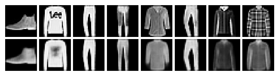
Reconstruction starts from a real image \(\boldsymbol{x}\), encodes it through \(q_\phi(\boldsymbol{z}|\boldsymbol{x})\), samples or uses a representative latent code, and decodes it back to an image. This checks whether the encoder-decoder pair can preserve the information needed to explain observed data. Good reconstructions indicate that the latent channel and decoder are expressive enough. Poor reconstructions may indicate an overly tight bottleneck, an undertrained decoder, an unsuitable likelihood model, or too much KL pressure.
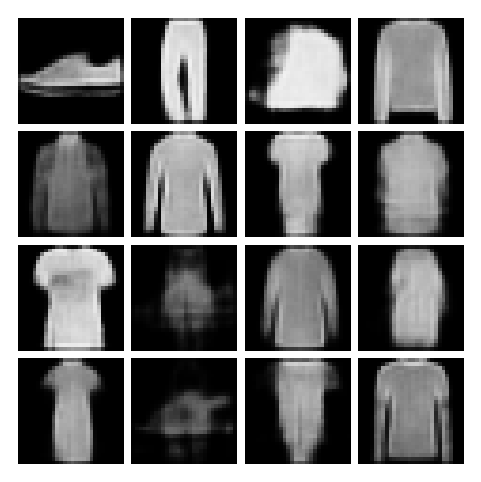
Generation starts from the prior, usually \(\boldsymbol{z}\sim\mathcal{N}(\boldsymbol{0},\boldsymbol{I})\), and decodes the sampled latent variables. This checks whether the learned decoder works on the regions of latent space that will actually be visited at sampling time. This is different from reconstruction. A model can reconstruct well using latent codes produced by the encoder, yet generate poorly if the aggregate posterior does not match the prior. Prior samples therefore test the generative model itself, not only the autoencoding path.
Interpolation takes two encoded images and moves between their latent representations before decoding each intermediate point. This checks the geometry of the latent space. If interpolation produces gradual semantic changes, the model has learned a latent organization in which nearby points decode to related images. If interpolation jumps abruptly, passes through unrealistic images, or changes unrelated factors erratically, the latent space is less coherent. Interpolation is not a proof that the true data manifold has been recovered, but it is a useful diagnostic of whether the learned representation is smooth and semantically meaningful.
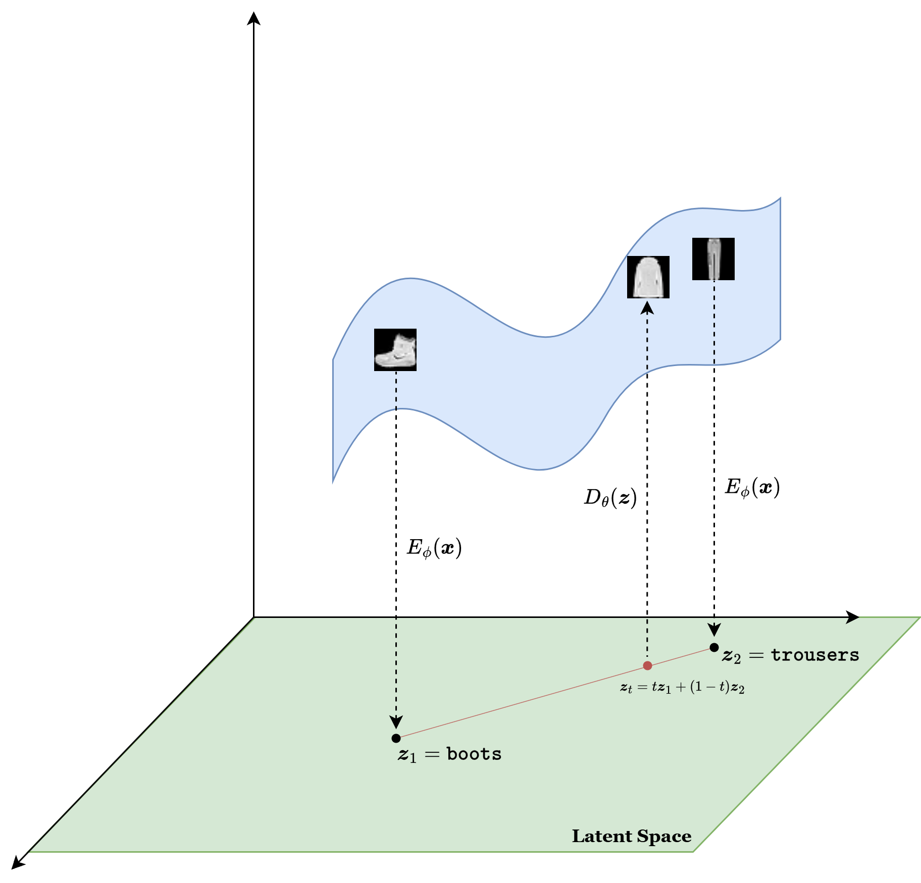
Fig. 18 The VAE interpolation mechanism.#
These three experiments answer different questions. Reconstruction asks whether information can pass through the latent bottleneck. Generation asks whether sampling from the prior produces plausible new images. Interpolation asks whether the latent space has a usable geometry.
Diagnostic meaning
Reconstruction checks information flow through the latent bottleneck. Generation checks whether prior samples decode to plausible images. Interpolation checks whether the latent space has a smooth and meaningful geometry.
Reconstructions, Samples, and Latent Geometry#
A VAE should be read through several lenses at once. Reconstructions tell us whether the encoder-decoder pair is transmitting enough information. Prior samples tell us whether the learned latent space remains compatible with the prior we want to sample from. Interpolations tell us whether the latent space has acquired a reasonably smooth semantic geometry rather than becoming a disconnected codebook.
@torch.no_grad()
def show_reconstructions(model, loader, device, n=8):
    model.eval()
    x, _ = next(iter(loader))
    x = x[:n].to(device)
    logits, _, _ = model(x)
    # Sigmoid is only for visualization; training used logits directly.
    recon = torch.sigmoid(logits).view(-1, 1, 28, 28)

    grid = torch.cat([x.cpu(), recon.cpu()], dim=0)
    image = utils.make_grid(grid, nrow=n, pad_value=1.0)
    plt.figure(figsize=(1.5 * n, 3.0))
    plt.imshow(image.permute(1, 2, 0), cmap="gray")
    plt.axis("off")
    plt.show()


@torch.no_grad()
def show_samples(model, device, n=16):
    model.eval()
    z = torch.randn(n, latent_dim, device=device)
    logits = model.decode(z)
    samples = torch.sigmoid(logits).view(-1, 1, 28, 28).cpu()
    image = utils.make_grid(samples, nrow=4, pad_value=1.0)
    plt.figure(figsize=(6, 6))
    plt.imshow(image.permute(1, 2, 0), cmap="gray")
    plt.axis("off")
    plt.show()

show_reconstructions(model, test_loader, device)
show_samples(model, device)
@torch.no_grad()
def interpolate(model, loader, device, steps=8):
    model.eval()
    x, _ = next(iter(loader))
    x0 = x[0:1].to(device)
    x1 = x[1:2].to(device)

    # Interpolate between posterior means to visualize latent geometry.
    mu0, _ = model.encode(x0)
    mu1, _ = model.encode(x1)

    alphas = torch.linspace(0, 1, steps, device=device).view(-1, 1)
    z = (1 - alphas) * mu0 + alphas * mu1
    logits = model.decode(z)
    images = torch.sigmoid(logits).view(-1, 1, 28, 28).cpu()

    grid = utils.make_grid(images, nrow=steps, pad_value=1.0)
    plt.figure(figsize=(1.7 * steps, 2.5))
    plt.imshow(grid.permute(1, 2, 0), cmap="gray")
    plt.axis("off")
    plt.show()


interpolate(model, test_loader, device)

Interpolation is particularly revealing when discussing the relation between VAEs and the manifold hypothesis. If linear motion in latent space produces gradual semantic motion in image space, that is evidence that the model has learned a coordinate system with some geometric coherence. It does not prove that the latent space is the true data manifold, but it does show that the model is organizing variation in a more structured way than raw pixel space does.
Quantitative Evaluation#
Visual inspection is necessary but incomplete. FID and KID compare real and generated images in a feature space, giving a distribution-level diagnostic. For a VAE, these metrics are especially useful because reconstruction quality can look acceptable even when prior samples are weak. The model may know how to decode latent points produced by the encoder while still behaving poorly on latent points sampled directly from the prior.
def prepare_for_inception_metrics(images):
    # The default Inception feature extractor expects RGB-like inputs.
    if images.size(1) == 1:
        images = images.repeat(1, 3, 1, 1)
    return images.clamp(0.0, 1.0)


@torch.no_grad()
def compute_vae_fid_and_kid(model, real_loader, device, num_fake=1000, metric_batch_size=64):
    fid = FrechetInceptionDistance(
        feature=2048,
        normalize=True,
        reset_real_features=False,
    ).set_dtype(torch.float64).to(device)
    kid = KernelInceptionDistance(
        feature=2048,
        subsets=10,
        subset_size=100,
        normalize=True,
        reset_real_features=False,
    ).to(device)

    # First accumulate features from real images in small batches.
    seen_real = 0
    real_target = num_fake
    for real_images, _ in tqdm(real_loader, desc="VAE real metrics", leave=False):
        remaining = real_target - seen_real
        if remaining <= 0:
            break
        real_images = real_images[: min(metric_batch_size, remaining)].to(device)
        real_images = prepare_for_inception_metrics(real_images)
        fid.update(real_images, real=True)
        kid.update(real_images, real=True)
        seen_real += real_images.size(0)

    # Then accumulate features from generated samples.
    generated = 0
    pbar = tqdm(total=num_fake, desc="VAE fake metrics", leave=False)
    while generated < num_fake:
        batch_n = min(metric_batch_size, num_fake - generated)
        z = torch.randn(batch_n, latent_dim, device=device)
        logits = model.decode(z)
        fake_images = torch.sigmoid(logits).view(-1, 1, 28, 28)
        fake_images = prepare_for_inception_metrics(fake_images)
        fid.update(fake_images, real=False)
        kid.update(fake_images, real=False)
        generated += batch_n
        pbar.update(batch_n)
    pbar.close()

    kid_mean, kid_std = kid.compute()
    return {
        "fid": fid.compute().item(),
        "kid_mean": kid_mean.item(),
        "kid_std": kid_std.item(),
    }


metric_scores = compute_vae_fid_and_kid(model, test_loader, device)
print(metric_scores)
c:\Users\tivog\deep-generative-models\.venv\lib\site-packages\torchmetrics\utilities\prints.py:43: UserWarning: Metric `Kernel Inception Distance` will save all extracted features in buffer. For large datasets this may lead to large memory footprint.
  warnings.warn(*args, **kwargs)
{'fid': 86.49043233491733, 'kid_mean': 0.06395631283521652, 'kid_std': 0.005002717953175306}
This evaluation block also clarifies one of the VAE’s characteristic tradeoffs. A VAE may reconstruct cleanly and organize latent space nicely, yet still obtain weaker FID or KID than a sharper generator because the decoded samples can look slightly smooth or blurry in feature space. That does not make the model useless. It means the metric is emphasizing a specific aspect of generative quality, namely closeness of the generated feature distribution to the real one.
Vanilla VAE Limitations#
The derivation above reveals why vanilla VAEs have characteristic limitations.
The first issue is the balancing problem. The reconstruction term asks the latent code to carry information that helps reproduce the image. The KL term asks the approximate posterior to remain close to the simple prior. Both forces are necessary, but they pull in different directions. If reconstruction dominates, the model may behave like a noisy autoencoder whose latent distribution is hard to sample from. If the KL term dominates, the latent channel may carry too little information.
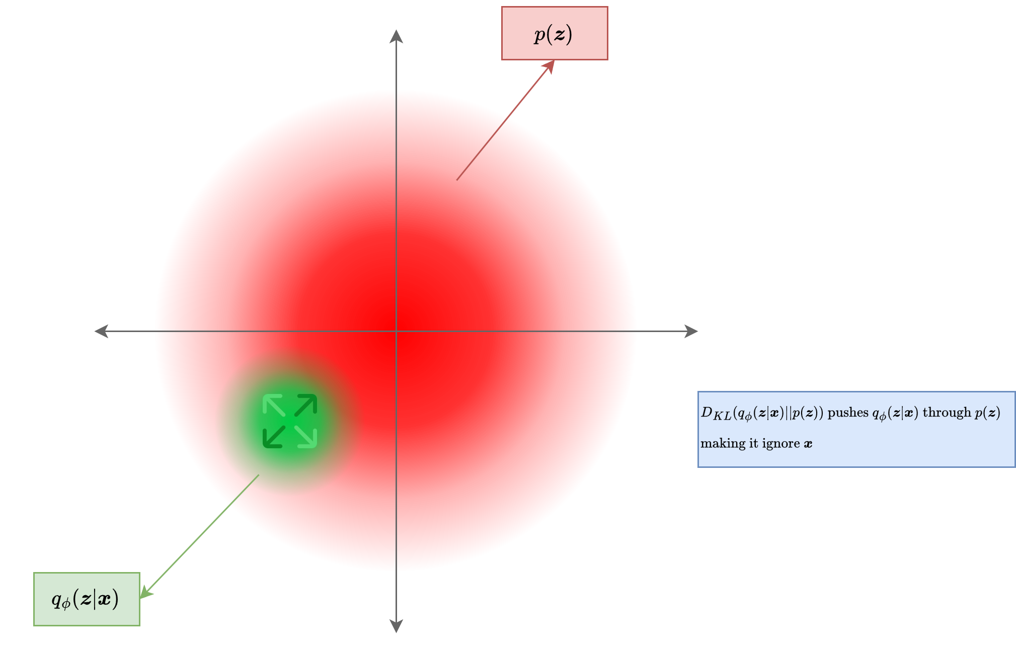
Fig. 19 Mode collapse happens because the \(D_{KL}\) term is too strong.#
The second issue is posterior collapse. In this failure mode, the encoder outputs a posterior close to the prior for many inputs, so the decoder receives almost no input-specific information from \(\boldsymbol{z}\). A coordinate-wise version is a dead latent dimension: one coordinate remains distributed nearly as standard normal noise regardless of the image. The coordinate exists in the architecture, but it transmits essentially no information.
The third issue is aggregate posterior versus prior mismatch. The ELBO regularizes each per-image posterior \(q_\phi(\boldsymbol{z}|\boldsymbol{x})\) toward \(p(\boldsymbol{z})\), but generation samples from the prior directly. What matters for sampling is whether the encoded population, averaged over the data distribution, occupies the same regions as the prior. Good reconstructions do not automatically imply good prior samples.
The fourth issue is blurriness. Pixelwise likelihoods such as Bernoulli or Gaussian decoders reward safe averages when the conditional output is ambiguous. If several sharp images are plausible under a latent code, their average may have good pixelwise likelihood but poor perceptual quality. This is one reason VAE variants explore richer decoders, learned priors, hierarchical latents, perceptual losses, adversarial losses, and modified KL schedules. The survey by Asperti, Evangelista, and Loli Piccolomini [AELP21] organizes many such variants around these limitations and their computational cost.
Main VAE tension
The same KL term that makes prior sampling meaningful can also restrict the information carried by \(\boldsymbol{z}\). This is the source of the reconstruction-sampling tradeoff, posterior collapse, and the need for KL-weight variants.
Theorem 10 (Expected KL as information plus prior mismatch)
Let \(p_{gt}(\boldsymbol{x})\) be the data distribution, let \(q_\phi(\boldsymbol{z} | \boldsymbol{x})\) be the encoder, and define the aggregate posterior
Then
where \(I_q(\boldsymbol{x};\boldsymbol{z})\) is the mutual information under the joint distribution \(p_{gt}(\boldsymbol{x})q_\phi(\boldsymbol{z} | \boldsymbol{x})\).
Proof. Start from the expected KL term and insert the aggregate posterior:
Multiply and divide inside the logarithm by \(q_\phi(\boldsymbol{z})\):
The first integral is exactly the mutual information between \(\boldsymbol{x}\) and \(\boldsymbol{z}\) under the encoder joint. In the second integral, integration over \(\boldsymbol{x}\) turns \(p_{gt}(\boldsymbol{x})q_\phi(\boldsymbol{z} | \boldsymbol{x})\) into \(q_\phi(\boldsymbol{z})\), giving the KL divergence between the aggregate posterior and the prior.
This theorem is a useful diagnostic lens. The average KL term is not a single monolithic penalty. It simultaneously controls how much information the latent variable carries about the input and how closely the encoded population matches the prior used at sampling time. Posterior collapse corresponds to the information term becoming too small. Poor prior samples can arise when the aggregate-posterior mismatch remains large even though reconstructions look acceptable. Many VAE variants can be read as attempts to control one side of this decomposition more precisely.
The broader lesson is that a VAE is best understood as a coupled system: probabilistic assumptions, latent geometry, decoder likelihood, inference approximation, and optimization all interact. Changing the KL weight, latent dimension, decoder capacity, or observation model changes the balance between reconstruction, sample quality, and latent usage.
The VAE is the canonical bridge between probabilistic latent-variable modeling and neural network autoencoding. It begins as a maximum-likelihood problem, becomes difficult because marginalization and posterior inference are intractable, introduces a variational posterior to obtain the ELBO, and finally takes the shape of a stochastic autoencoder trained by reparameterized gradients. Its limitations are not failures of the derivation. They are the visible consequences of the approximations that make the model trainable.