
Discrete Diffusion Models#
Diffusion models return to an explicitly probabilistic style of reasoning, but they do so through a very different latent construction from VAEs. Instead of introducing a single latent code \(\boldsymbol{z}\), they introduce an entire trajectory \(\boldsymbol{x}_0, \boldsymbol{x}_1, \ldots, \boldsymbol{x}_T\), where \(\boldsymbol{x}_0\) is the clean image and the later variables are progressively corrupted versions of it. The central formulation of modern discrete diffusion models is due to Sohl-Dickstein et al. [SDWMG15] and was turned into the DDPM training recipe by Ho, Jain, and Abbeel [HJA20].
The key modeling move is to decompose generation into many small denoising corrections. Instead of asking a network to map one latent vector directly into a full image, diffusion asks it to invert a long sequence of tiny Gaussian corruption steps. Each individual reverse step is simple enough that it can be modeled with stable regression-style objectives, and the global generative process emerges from the repeated composition of those local denoising updates.
The transition from GANs to diffusion is one of the sharpest conceptual shifts in modern generative modeling. GANs demonstrated that excellent samples can arise from an implicit model trained by an adaptive critic, but they also exposed how difficult unstable game optimization can be in high dimension. Diffusion responds by changing not only the loss, but the granularity of the generative task itself. Rather than learning one direct jump from latent noise to image space, it learns how to reverse a carefully designed stochastic process. This design is the main reason diffusion training often behaves much more like a supervised learning problem than an adversarial one.
There is a useful contrast with VAEs. A VAE introduces one latent variable and then spends most of its effort dealing with posterior intractability. A diffusion model takes the opposite path: it introduces a very large number of latent variables, one for each noise level in the chain, but chooses the forward process so carefully that many of the relevant Gaussian quantities become analytically tractable. The resulting model is therefore more elaborate in latent structure but, in some sense, simpler in local conditional algebra. This is one reason diffusion models often feel paradoxical at first: they are conceptually deeper than a vanilla autoencoder, yet some of their core training identities are easier to manipulate once the forward process has been designed.
It is also helpful to say explicitly what problem diffusion is solving compared with GANs. GANs try to learn a direct path from latent noise to realistic images through a learned adversarial game, and their difficulty lies largely in unstable optimization. Diffusion chooses a much longer route. It asks the model to solve many easy denoising problems instead of one hard synthesis problem. The price is sampling cost. The reward is a training objective that behaves much more like a supervised regression problem. Much of the modern success of diffusion models comes from this tradeoff.
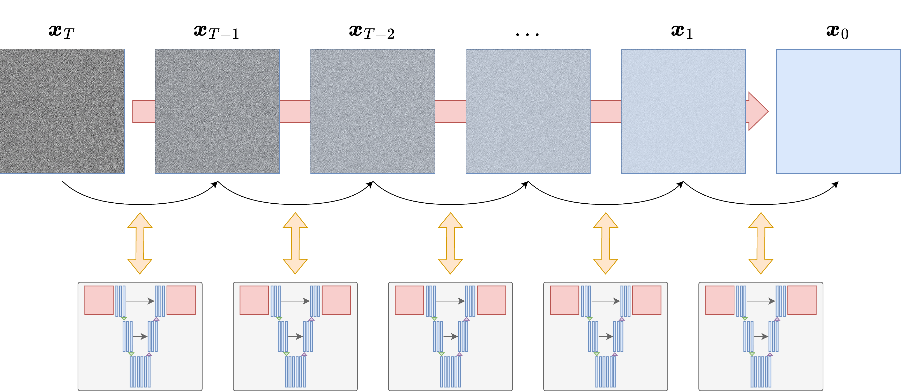
Fig. 33 A conceptual diagram of the diffusion-model viewpoint: a forward noising path and a learned reverse denoising path.#
Important
The central diffusion idea is decomposition. Instead of learning one global jump from noise to image, the model learns many local denoising steps. That is the main reason the objective becomes stable enough to train at scale.
The Forward Noising Process#
Let \(\boldsymbol{x}_0 \sim p_{gt}\) be a data sample. The forward process is a Markov chain
where each transition adds a small amount of Gaussian noise:
The sequence \(\beta_t \in (0,1)\) is the noise schedule. When \(\beta_t\) is small, the transition only perturbs the image slightly. Repeating this many times gradually destroys structure until the terminal variable \(\boldsymbol{x}_T\) is close to an isotropic Gaussian. It is useful to introduce one more quantity:
With this notation, \(\bar{\alpha}_t\) is the local one-step signal retention, while \(\alpha_t\) is the cumulative signal retention after \(t\) noising steps. This discrete construction is the one used in DDPMs [HJA20].
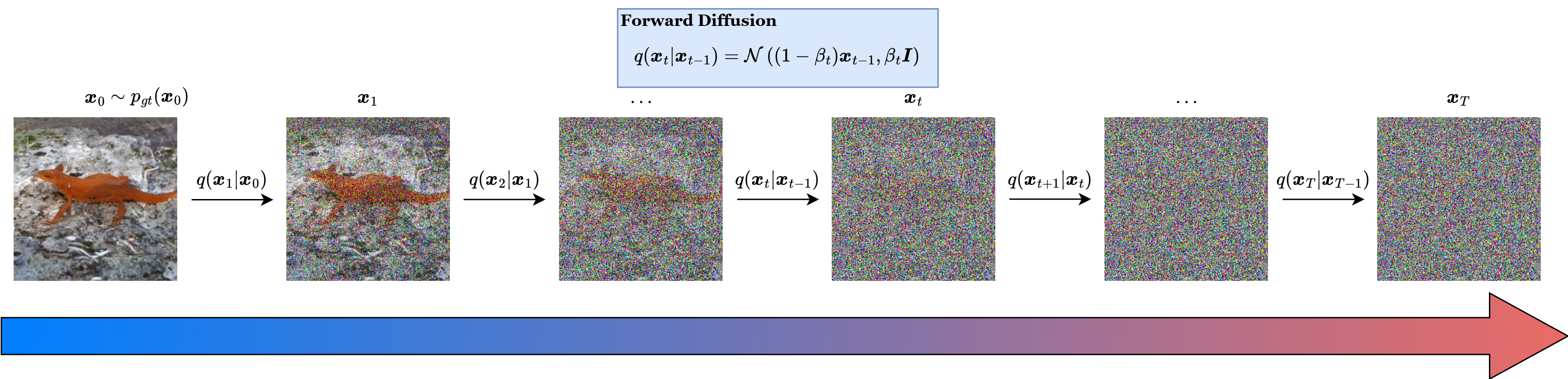
Fig. 34 In the forward noising process, an input image gets increasingly corrupted with noise while reducing the amount of image signal.#
Theorem 13 (Closed form of the forward marginal)
For every \(t \in \{1,\ldots,T\}\),
Equivalently,
Proof. We proceed by induction on \(t\). For \(t=1\), the formula is immediate because \(\alpha_1 = \bar{\alpha}_1\) and
Assume the statement holds at time \(t-1\), so that
for a standard Gaussian \(\boldsymbol{\varepsilon}_{t-1}\). The next transition gives
Substituting the induction hypothesis,
The last two terms are independent centered Gaussians, so their sum is again Gaussian with covariance
Since \(\bar{\alpha}_t\alpha_{t-1} = \alpha_t\), the claim follows.
This theorem is one of the reasons diffusion models are computationally practical. It says that one does not need to simulate the entire forward chain to sample a noisy observation at time \(t\). A draw from \(q(\boldsymbol{x}_t | \boldsymbol{x}_0)\) can be generated directly in one step. During training, this makes it possible to choose a random time index and generate the corresponding noisy sample without unrolling all earlier transitions.
A concrete image example helps. If \(\boldsymbol{x}_0\) is a clean handbag image and \(t\) is small, the corresponding \(\boldsymbol{x}_t\) still looks like the same handbag with a light dusting of Gaussian corruption. If \(t\) is large, the shape is barely recognizable and the sample is close to pure static. Training asks one network to operate across this whole range of difficulty.
Numerical Example: How Much Signal Survives?
Take a toy noise schedule with \(\beta_1 = 0.1\) and \(\beta_2 = 0.2\). Then \(\bar{\alpha}_1 = 0.9\), \(\bar{\alpha}_2 = 0.8\), and \(\alpha_2 = 0.9 \cdot 0.8 = 0.72\). The closed-form forward marginal says
Numerically, \(\sqrt{0.72} \approx 0.849\) and \(\sqrt{0.28} \approx 0.529\). So after only two steps, about eighty-five percent of the original signal amplitude is still present, but a substantial noise term has already been mixed in.
Early diffusion steps do not destroy the image completely. They weaken the signal gradually while increasing uncertainty, which is exactly why the reverse denoiser can hope to recover the structure one small step at a time.
Conceptually, the theorem also explains why diffusion training can be randomized over time in such a simple way. The network does not need to see only neighboring states such as \(\boldsymbol{x}_{t-1}\) and \(\boldsymbol{x}_t\). Because \(\boldsymbol{x}_t\) has a direct closed form given \(\boldsymbol{x}_0\), the algorithm can choose a random noise level and present the model with the corresponding corrupted example immediately. This makes the training loop look much closer to ordinary supervised learning than one might expect from the long latent trajectory written in the model definition.
A useful interpretation is that \(\alpha_t\) measures how much signal survives by time \(t\), while \(1-\alpha_t\) measures how much isotropic Gaussian corruption has been accumulated. Early times correspond to a slightly perturbed image. Late times correspond to something close to pure noise. The network is therefore exposed to a curriculum of denoising subproblems indexed by noise scale.
The Reverse Process#
The forward chain is fixed and easy to sample from. The generative task is to learn a reverse chain
where \(p(\boldsymbol{x}_T)\) is chosen to be a standard Gaussian and each reverse transition is modeled as
The neural network is therefore asked to undo one infinitesimal corruption step at a time. This local formulation is crucial. Directly generating a realistic image from white noise in one step is very hard. Predicting how to remove a little amount of Gaussian corruption from a partially structured image is far more manageable, and this is exactly the principle that makes DDPMs effective [HJA20].
One way to read this model is as a chain of microscopic decoders. Each reverse conditional takes a slightly too noisy image and tries to move it one step closer to the data manifold. No single step is responsible for creating the whole image. Global structure emerges cumulatively from the repeated composition of local denoising moves. This is very different from the generator in a GAN, which must learn a direct global transport from latent noise to the image space in one pass.
This local perspective is also why U-Nets become such a natural architecture for diffusion. At intermediate times, the input to the network already contains a coarse version of the eventual image, buried under noise. The model does not need to invent all structure from scratch; it needs to preserve what is reliable, infer what is ambiguous, and progressively sharpen detail across scales. Architecturally, that is exactly the sort of task for which multi-scale skip-connected networks are well suited.
Approximating the Reverse Process with a Neural Network#
To learn the reverse chain, one needs to understand the exact Gaussian posterior
If both the clean image \(\boldsymbol{x}_0\) and the noisy image \(\boldsymbol{x}_t\) are known, then the previous state \(\boldsymbol{x}_{t-1}\) is constrained by two linear Gaussian relations, so the posterior can still be computed in closed form. The next theorem gives the exact target that the learned reverse conditional is trying to approximate.
Theorem 14 (Closed form of the forward posterior)
For the Gaussian forward process
with cumulative coefficient \(\alpha_t=\prod_{s=1}^{t}\bar{\alpha}_s\), the posterior of one previous noisy state conditioned on \(\boldsymbol{x}_t\) and \(\boldsymbol{x}_0\) is
where
and
Proof. The posterior is proportional to the product of two Gaussian factors:
The first factor is
and the forward-marginal theorem gives
Multiplying the two Gaussian densities as functions of \(\boldsymbol{x}_{t-1}\) gives another Gaussian. Completing the square in \(\boldsymbol{x}_{t-1}\) yields the covariance
and the corresponding mean is
This proves the stated posterior formula.
This posterior formula makes diffusion models look strikingly close to latent-variable models. The forward chain defines a tractable encoder-like distribution \(q\). The reverse chain defines a learned decoder-like distribution \(p_\theta\). The main difference from a VAE is that the latent structure is not a single vector but a long Markov chain whose conditionals have been chosen to admit closed-form Gaussian manipulations.
This posterior formula makes the approximation problem unusually concrete. The network is not trying to mimic an arbitrary unknown conditional distribution. It is trying to infer the mean of a known Gaussian family from the pair \((\boldsymbol{x}_t, t)\) alone. Once the forward chain has been fixed analytically, the modeling freedom is concentrated almost entirely in this denoising map.
It is worth stressing how unusual this design choice is. In a VAE, the variational distribution is learned because the exact posterior is too hard to compute. In DDPMs, much of the posterior structure is known analytically because the forward corruption was fixed in advance. The modeling freedom is moved away from the encoder side and concentrated in the reverse denoiser. This is one of the deepest structural differences between the two families, even though both are trained through an ELBO.
The theorem also clarifies why the reverse model is asked to predict relatively simple Gaussian statistics rather than an arbitrary conditional density. Once the forward chain is chosen, the true reverse posterior conditioned on \(\boldsymbol{x}_0\) is already Gaussian. The learning problem becomes: can a neural network infer the right Gaussian mean, or an equivalent target such as the added noise, from the noisy image and the time index alone?
ELBO Loss#
The log-likelihood of the model can be lower bounded using the forward process as a variational distribution. Starting from
we multiply and divide by \(q(\boldsymbol{x}_{1:T} | \boldsymbol{x}_0)\) and apply Jensen’s inequality exactly as in the VAE derivation. This yields the evidence lower bound
After expanding the Markov factorizations and regrouping terms, one obtains a sum of Kullback-Leibler divergences between exact forward posteriors and learned reverse transitions, plus a terminal prior matching term and a reconstruction term at time \(t=1\). This is the discrete-diffusion ELBO derived in the DDPM literature [HJA20].
Theorem 15 (ELBO decomposition for discrete diffusion)
Up to sign conventions, the negative ELBO can be decomposed as
Proof. Expand the ELBO integrand using
and
Rearranging the resulting sum and repeatedly inserting
produces one KL term for each reverse step, one KL term matching the terminal marginal to the chosen Gaussian prior, and one data reconstruction term involving \(p_\theta(\boldsymbol{x}_0 | \boldsymbol{x}_1)\). The proof is structurally the same as in variational latent-variable models, except that the latent space is now the entire trajectory.
The importance of this theorem is conceptual. A DDPM can be viewed as a very deep latent-variable model whose latent variables are the noisy intermediate states. The forward process plays the role of an analytically chosen inference model, while the reverse chain is learned. This is precisely why the connection with VAEs is not superficial. Both methods optimize a variational lower bound. They differ mainly in how the latent structure is designed and in how expressive the reverse conditionals become when the number of steps is large.
This VAE connection deserves to be made even more explicit. If one writes the VAE ELBO schematically, one sees a reconstruction term plus a regularization term that compares an approximate posterior with a prior. In diffusion, the same broad logic survives, but it is distributed across time. Each KL term compares one exact local reverse posterior from the forward process with one learned local reverse conditional. Instead of asking one latent variable to summarize the whole image, the model asks a long chain of noisy latents to carry the information gradually. The gain is that each local denoising task is simple. The cost is that generation becomes iterative.
VAEs and DDPMs therefore make two different tractability choices. VAEs keep sampling cheap but inference approximate. Diffusion keeps local posterior algebra easy but sampling long. Much of modern generative modeling can be read as a sequence of such redistributions of difficulty rather than as a complete removal of difficulty.
Noise Prediction Parameterization#
The reverse mean can be parameterized in several equivalent ways. One especially successful choice is to make the neural network predict the noise \(\boldsymbol{\varepsilon}\) used to generate \(\boldsymbol{x}_t\) from \(\boldsymbol{x}_0\). From the forward marginal identity,
one can solve for \(\boldsymbol{x}_0\):
If a network \(\boldsymbol{\varepsilon}_\theta(\boldsymbol{x}_t, t)\) predicts the noise, then this estimate can be substituted into the posterior mean formula. After fixing the reverse variance to a known schedule, the corresponding KL term reduces to a weighted mean squared error between the true noise and the predicted noise. This is the parameterization that made DDPMs practical to optimize at scale [HJA20].
In many practical expositions, the training objective is therefore written in the simplified form
where
A complicated variational objective is therefore turned into a denoising regression problem that is easy to implement and optimize. Later, in score-based models, predicting the noise will reappear as a reparameterized form of score prediction.
The simplification above is not merely a coding convenience. It changes the way one should interpret the method. The network is no longer viewed primarily as a density model in the classical sense. It becomes a time-conditioned denoiser trained across many corruption scales. The probabilistic interpretation remains essential, because it explains why this denoising regression objective is legitimate, but the optimization face of the model is strikingly close to supervised learning on synthetic noisy targets.
This is one reason diffusion models were comparatively easy to scale once the architectural ingredients became available. Deep learning already knows how to fit large regression networks well. If one can reformulate generative modeling so that the central neural task is “predict the noise that was added,” a great deal of existing optimization machinery becomes immediately useful.
DDPM Sampling#
The training objective explains how the network is fitted. Sampling explains how the network is used. Starting from \(\boldsymbol{x}_T \sim \mathcal{N}(\boldsymbol{0}, \boldsymbol{I})\), the reverse process repeatedly predicts what the clean image should be and then moves one step toward that cleaner image.
Given a noisy sample \(\boldsymbol{x}_t\), the denoiser predicts \(\boldsymbol{\varepsilon}_\theta(\boldsymbol{x}_t, t)\). From that prediction one forms the standard estimate
This is the model’s guess of the underlying clean image that gave rise to the current noisy state. The full ancestral DDPM sampling rule is the one introduced in [HJA20].
That estimate is then injected into the reverse posterior mean:
Sampling uses
with the stochastic term omitted at the final step. This is the core DDPM intuition: estimate the clean image hidden inside the noise, then step to a slightly less noisy state, then repeat.
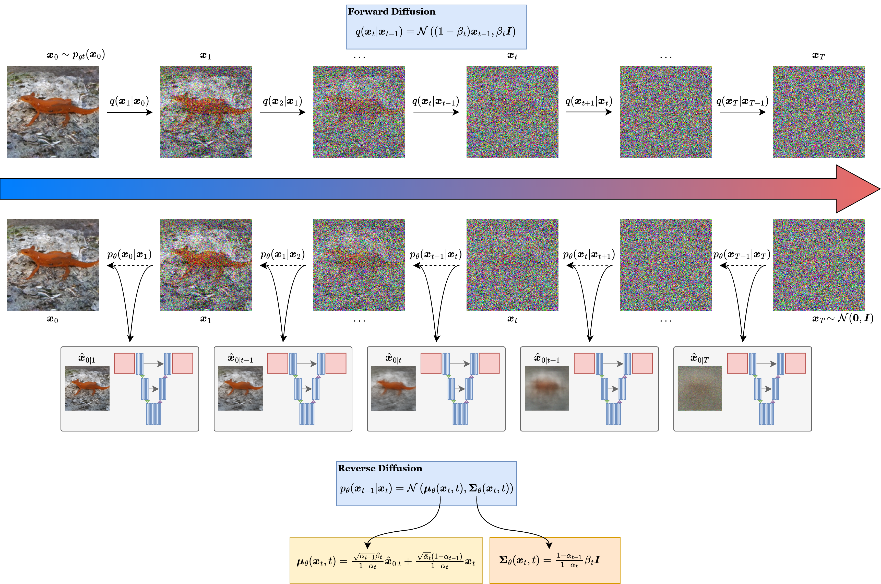
Fig. 35 In the backward denoising process, pure noise gets iteratively denoised by alternatively applying a denoiser neural network to compute \(\hat{\boldsymbol{x}}_{0 | t}\) from \(\boldsymbol{x}_t\), and then re-corrupting it by adding noise with lower noise level.#
Numerical Example: One Reverse Step
Suppose \(t\) is late in the chain, so \(\boldsymbol{x}_t\) is heavily corrupted. The denoiser sees that noisy image and predicts the noise component that was likely added. Subtracting that estimated noise gives \(\hat{\boldsymbol{x}}_{0|t}\), a provisional clean-image estimate. The reverse posterior mean then combines the current \(\boldsymbol{x}_t\) and this clean estimate into the center of a Gaussian for \(\boldsymbol{x}_{t-1}\). A fresh Gaussian draw adds only a small amount of uncertainty back, because \(\boldsymbol{x}_{t-1}\) should be slightly less noisy than \(\boldsymbol{x}_t\).
DDIM Sampling#
The training objective of DDIM is the same as the training objective of DDPM. The forward noising process is the same, the denoiser is the same, and the noise-prediction network is trained in exactly the same way. The difference appears only at sampling time. DDIM reuses the same learned denoiser but follows a different reverse trajectory [SME21]. This is conceptually important. The network is not intrinsically tied to one unique reverse Markov chain. Once it can turn a noisy image \(\boldsymbol{x}_t\) into a good estimate \(\hat{\boldsymbol{x}}_{0|t}\), there is freedom in how the next less-noisy sample is constructed.
The DDIM update starts from the same estimate
It then defines a new sample at an earlier time \(t' < t\) by
The parameter \(\sigma_t\) controls how much randomness is injected. When \(\sigma_t = 0\), or equivalently when the common implementation parameter \(\eta = 0\), the update becomes deterministic once \(\boldsymbol{x}_T\) is fixed.
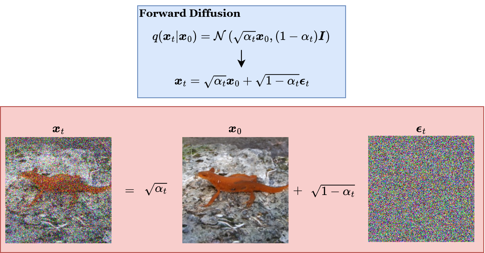
Fig. 36 A DDIM step uses the current noisy sample to estimate the clean image and then constructs a less noisy point on the same deterministic trajectory.#
This makes the DDIM intuition especially clean. At each stage, the denoiser takes a noisy image \(\boldsymbol{x}_t\), produces the implied clean-image estimate \(\hat{\boldsymbol{x}}_{0|t}\), and then reconstructs a slightly less noisy image \(\boldsymbol{x}_{t'}\) that is consistent with that estimate. One can describe the whole sampler informally as:
infer the clean image hidden inside the current noisy state;
re-add some noise, but less than before;
repeat on a coarser or finer time grid.
This is one of the most transparent ways to understand why diffusion models work at all.
A major practical advantage of DDIM is timestep skipping. The DDPM sampler usually runs through the entire sequence \(T, T-1, \ldots, 1\). DDIM often uses a subsequence such as
so only a smaller number of denoising evaluations is performed. The denoiser is still queried at real diffusion noise levels, but many intermediate levels are skipped during generation. This is one of the first places where diffusion becomes a story about model plus sampler, not only about the learned network. This is why DDIM became one of the first practically important accelerated samplers in the diffusion literature [SME21].
Note
With DDPM, the reverse chain remains stochastic even after \(\boldsymbol{x}_T\) is fixed, because fresh Gaussian noise is injected at each reverse step. With DDIM and \(\eta = 0\), the whole trajectory is deterministic once \(\boldsymbol{x}_T\) is fixed. Two runs started from the same terminal noise produce the same image.
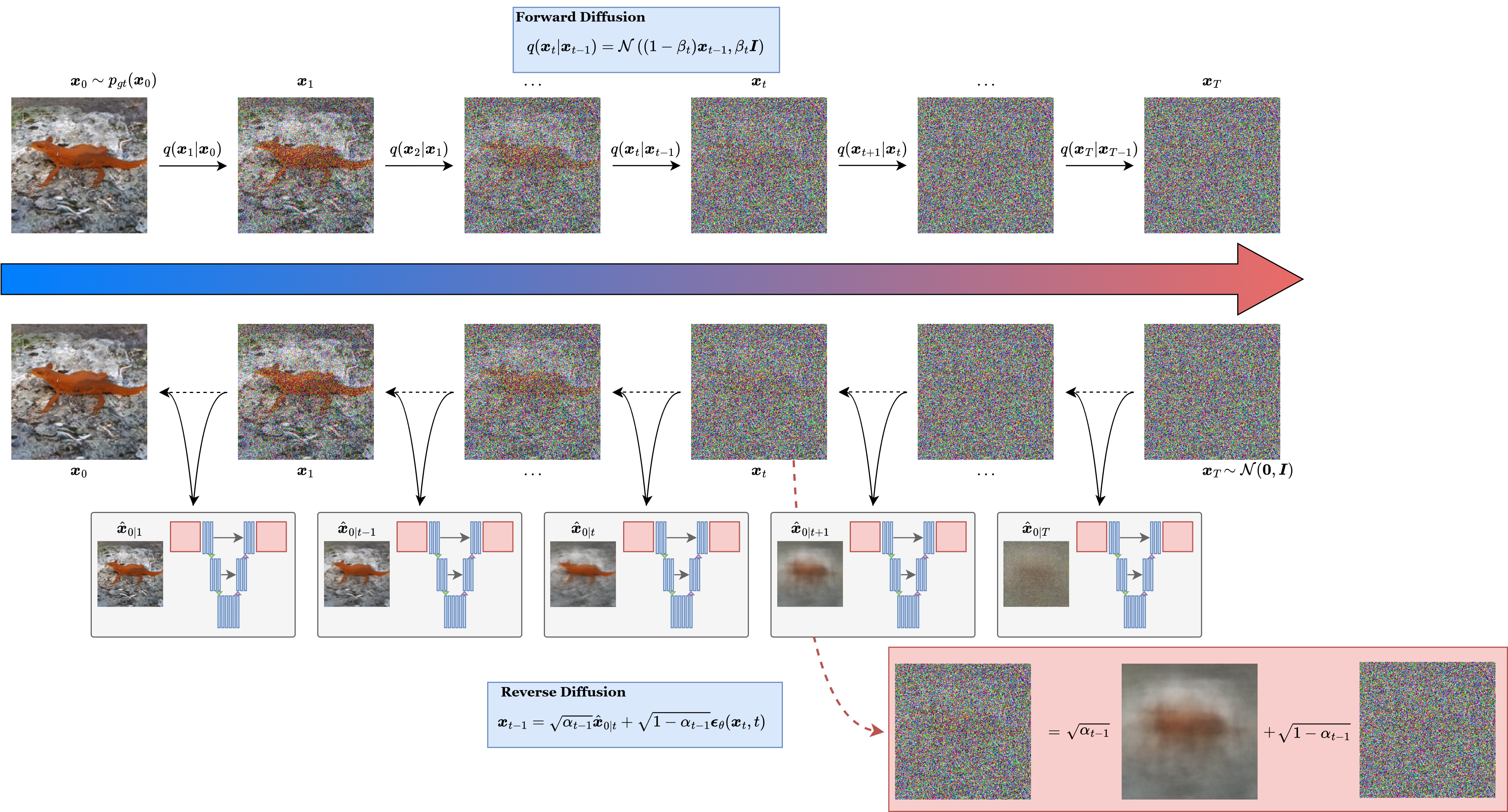
Fig. 37 DDIM backward process is the deterministic version of DDPM.#
Relation with VAEs, Latent Diffusion, and the Continuous-Time Limit#
It is worth closing the discrete discussion by clarifying the relation with the models studied earlier. A VAE learns a decoder from a compact latent code and must approximate the posterior because exact inference is hard. A discrete diffusion model chooses a much more elaborate latent structure, but in exchange the forward corruption process is analytically fixed and its marginals and local posteriors are tractable. The result is an optimization problem that remains variational in spirit while being unusually stable in practice.
Modern latent diffusion models add another twist to this story. Instead of running diffusion directly in pixel space, one first compresses images into a lower-dimensional latent representation using an autoencoding model, and then performs diffusion in that latent space. The motivation is computational rather than philosophical: denoising a compressed representation is dramatically cheaper than denoising full-resolution pixels, especially for high-resolution image synthesis. In this sense, latent diffusion can be viewed as a reconciliation between autoencoding ideas and diffusion ideas. The autoencoder provides a perceptually meaningful lower-dimensional space, and the diffusion model supplies the powerful generative prior inside that space [RBL+22].
When the number of diffusion steps becomes very large, the same ideas naturally lead to continuous-time stochastic dynamics written in terms of score matching, SDEs, and probability flow ODEs. The foundational DDPM perspective comes from [HJA20], while the deterministic-sampling and continuous-time viewpoints are developed in [SME21, SSDK+21].
Choosing the Noise Schedule#
The schedule is one of the first genuinely important design choices in a diffusion model. The local coefficient \(\beta_t\) decides how much variance is injected at step \(t\), while the cumulative coefficient \(\alpha_t\) determines how much of the original signal remains after many steps. If the schedule destroys structure too quickly, the denoiser must solve unnecessarily hard subproblems early in the chain. If it destroys structure too slowly, the terminal distribution may remain too far from a simple Gaussian and the reverse process may be inefficient.
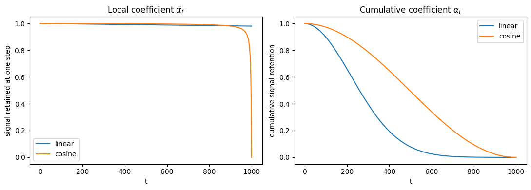
A good schedule aims for a smooth progression from “almost clean” images to “almost pure noise.” In early DDPM experiments, a linear schedule for \(\beta_t\) was common and already works well for compact settings [HJA20]. Later work introduced cosine schedules, which preserve useful signal for longer and often distribute the denoising difficulty more evenly across time [ND21]. In practice, the right schedule is not mysterious: it should make the path gradual, numerically stable, and long enough that the terminal distribution is simple.
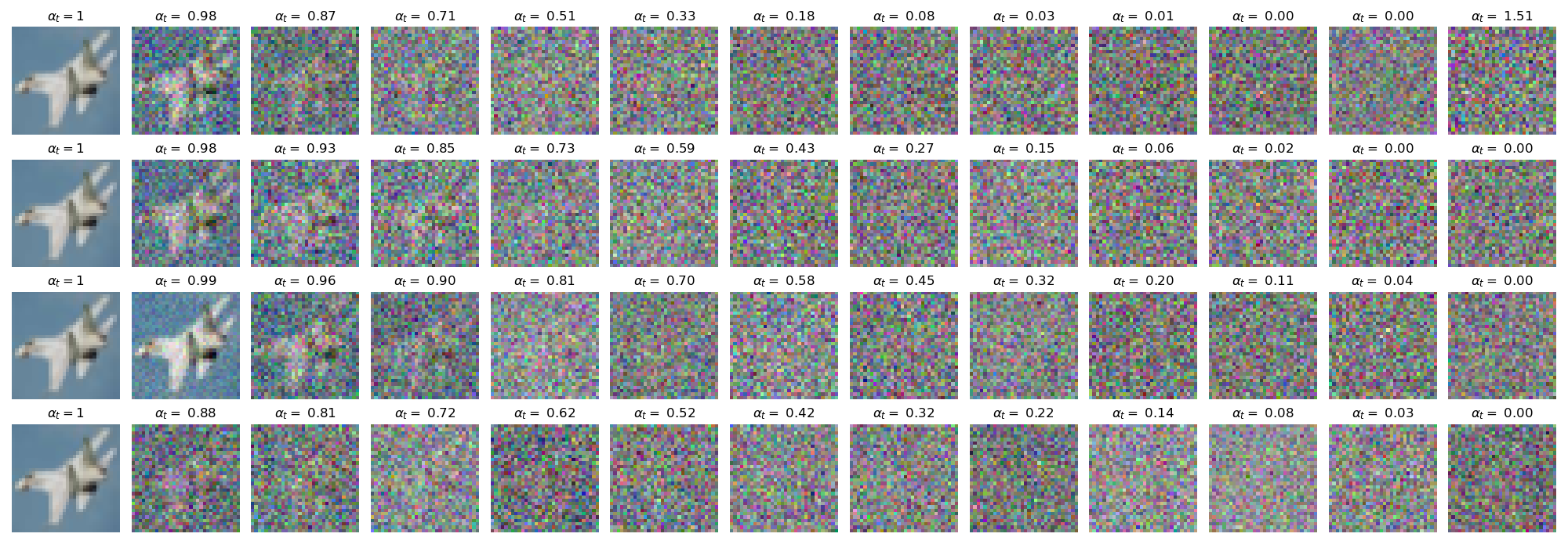
Fig. 38 The effect of different noise schedules on an input image.#
Note
A practical way to think about schedule design is to inspect the curve of \(\alpha_t\). If it collapses too quickly, the model spends too many steps near pure noise. If it stays too close to one for too long, the later reverse steps carry too much of the generative burden.
A short plotting routine makes this discussion concrete. The goal is not to commit immediately to one schedule, but to inspect how fast signal is removed and whether the cumulative curve decays smoothly or collapses too abruptly.
The snippet below compares a simple linear schedule with a standard cosine-inspired cumulative schedule. In practice, plots like these are often the quickest sanity check before training.
import math
import numpy as np
import matplotlib.pyplot as plt

T = 1000
steps = np.arange(1, T + 1)

# Linear beta schedule.
betas_linear = np.linspace(1e-4, 0.02, T)
bar_alphas_linear = 1.0 - betas_linear
alphas_linear = np.cumprod(bar_alphas_linear)

# Cosine-inspired cumulative schedule from Nichol and Dhariwal.
s = 0.008
t_grid = np.arange(T + 1) / T
f = np.cos(((t_grid + s) / (1 + s)) * math.pi / 2) ** 2
alphas_cosine = f[1:] / f[0]
bar_alphas_cosine = alphas_cosine / np.concatenate(([1.0], alphas_cosine[:-1]))

fig, axes = plt.subplots(1, 2, figsize=(11, 4))

axes[0].plot(steps, bar_alphas_linear, label="linear")
axes[0].plot(steps, bar_alphas_cosine, label="cosine")
axes[0].set_title(r"Local coefficient $\bar{\alpha}_t$")
axes[0].set_xlabel("t")
axes[0].set_ylabel("signal retained at one step")
axes[0].legend()

axes[1].plot(steps, alphas_linear, label="linear")
axes[1].plot(steps, alphas_cosine, label="cosine")
axes[1].set_title(r"Cumulative coefficient $\alpha_t$")
axes[1].set_xlabel("t")
axes[1].set_ylabel("cumulative signal retention")
axes[1].legend()

plt.tight_layout()
plt.show()
Guided DDPM Implementation#
At this point the probabilistic structure has a very direct code counterpart: the forward marginal, the noise schedule, the time conditioning, the denoiser, the noise-prediction loss, and the reverse samplers. The scale remains modest, but the algorithmic skeleton is the real one. The goal is to keep the model small enough to read line by line while preserving the actual structure of a DDPM and its DDIM variant. The implementation follows the modeling pattern introduced by Ho, Jain, and Abbeel [HJA20], with the practical schedule comparison informed by later refinements such as [ND21].
Imports, Dataset, and Practical Scale#
The implementation uses FashionMNIST. The denoiser is a small U-Net rather than a plain MLP, the number of diffusion steps is large enough to make the reverse process visibly iterative, and the training horizon is long enough that the denoising trajectory becomes recognizable.
import copy
import math
import torch
import torch.nn as nn
import torch.nn.functional as F
from pathlib import Path
from torch.utils.data import DataLoader
from torchmetrics.image.fid import FrechetInceptionDistance
from torchmetrics.image.kid import KernelInceptionDistance
from torchvision import datasets, transforms, utils
from tqdm.auto import tqdm
import matplotlib.pyplot as plt

device = torch.device("cuda" if torch.cuda.is_available() else "cpu")
torch.manual_seed(7)
if device.type == "cuda":
    torch.cuda.manual_seed_all(7)
num_workers = 0
project_root = Path.cwd() if (Path.cwd() / "_config.yml").exists() else Path.cwd().parent
DATA_ROOT = project_root / "data"

batch_size = 128
image_size = 28
channels = 1
base_channels = 64
time_dim = 128
timesteps = 300
epochs = 100
lr = 2e-4

transform = transforms.Compose([
    transforms.ToTensor(),
    transforms.Lambda(lambda x: 2.0 * x - 1.0),
])

train_dataset = datasets.FashionMNIST(
    root=DATA_ROOT,
    train=True,
    download=True,
    transform=transform,
)

train_loader = DataLoader(
    train_dataset,
    batch_size=batch_size,
    shuffle=True,
    num_workers=num_workers,
    pin_memory=(device.type == "cuda"),
)

artifacts_dir = project_root / "artifacts"
artifacts_dir.mkdir(exist_ok=True)
ddpm_checkpoint_path = artifacts_dir / "ddpm_fashionmnist.pt"
The main hyperparameters are worth reading as modeling commitments. The 300 diffusion steps create a reasonably fine noising curriculum while still keeping the reverse sampler manageable. The 50 training epochs are long enough that the model begins to produce images rather than merely proving that the code runs.
The Forward Process in Code#
The code below is the exact computational translation of the forward marginal theorem. The arrays betas, bar_alphas, and alphas are the schedule coefficients from the theory section, and q_sample implements the closed-form draw
\(\boldsymbol{x}_t = \sqrt{\alpha_t}\,\boldsymbol{x}_0 + \sqrt{1-\alpha_t}\,\boldsymbol{\varepsilon}\).
betas = torch.linspace(1e-4, 0.02, timesteps, device=device)
bar_alphas = 1.0 - betas
alphas = torch.cumprod(bar_alphas, dim=0)
alphas_prev = torch.cat([torch.tensor([1.0], device=device), alphas[:-1]], dim=0)

sqrt_alphas = torch.sqrt(alphas)
sqrt_one_minus_alphas = torch.sqrt(1.0 - alphas)
sqrt_recip_bar_alphas = torch.sqrt(1.0 / bar_alphas)
posterior_variance = betas * (1.0 - alphas_prev) / (1.0 - alphas)


def extract(coefficients, t, x_shape):
    out = coefficients.gather(0, t)
    return out.view(t.shape[0], *((1,) * (len(x_shape) - 1)))


def q_sample(x0, t, noise=None):
    if noise is None:
        noise = torch.randn_like(x0)
    return (
        extract(sqrt_alphas, t, x0.shape) * x0
        + extract(sqrt_one_minus_alphas, t, x0.shape) * noise
    )
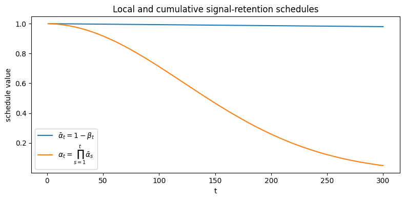
A schedule is easier to understand when it is plotted. The next cell visualizes both the local coefficient \(\bar{\alpha}_t = 1-\beta_t\) and the cumulative coefficient \(\alpha_t = \prod_{s=1}^t \bar{\alpha}_s\). The first stays close to one because each step only removes a small amount of signal. The second decays across time because those small losses accumulate.
steps = torch.arange(1, timesteps + 1)

plt.figure(figsize=(8, 4))
plt.plot(steps, bar_alphas.detach().cpu(), label=r"$\bar{\alpha}_t = 1-\beta_t$")
plt.plot(steps, alphas.detach().cpu(), label=r"$\alpha_t = \prod_{s=1}^t \bar{\alpha}_s$")
plt.xlabel("t")
plt.ylabel("schedule value")
plt.title("Local and cumulative signal-retention schedules")
plt.legend()
plt.tight_layout()
plt.show()
Time Conditioning and the Denoiser Architecture#
The network does not only see an image-like tensor. It must also know which noise level that tensor corresponds to. Time embeddings provide that context, and the U-Net-style architecture provides the multi-scale computation needed for denoising.
A raw integer time index is usually too crude a representation by itself. A sinusoidal embedding maps that scalar time into a vector of oscillatory features at multiple frequencies, so nearby times remain related while different time scales can still be distinguished clearly by the network.
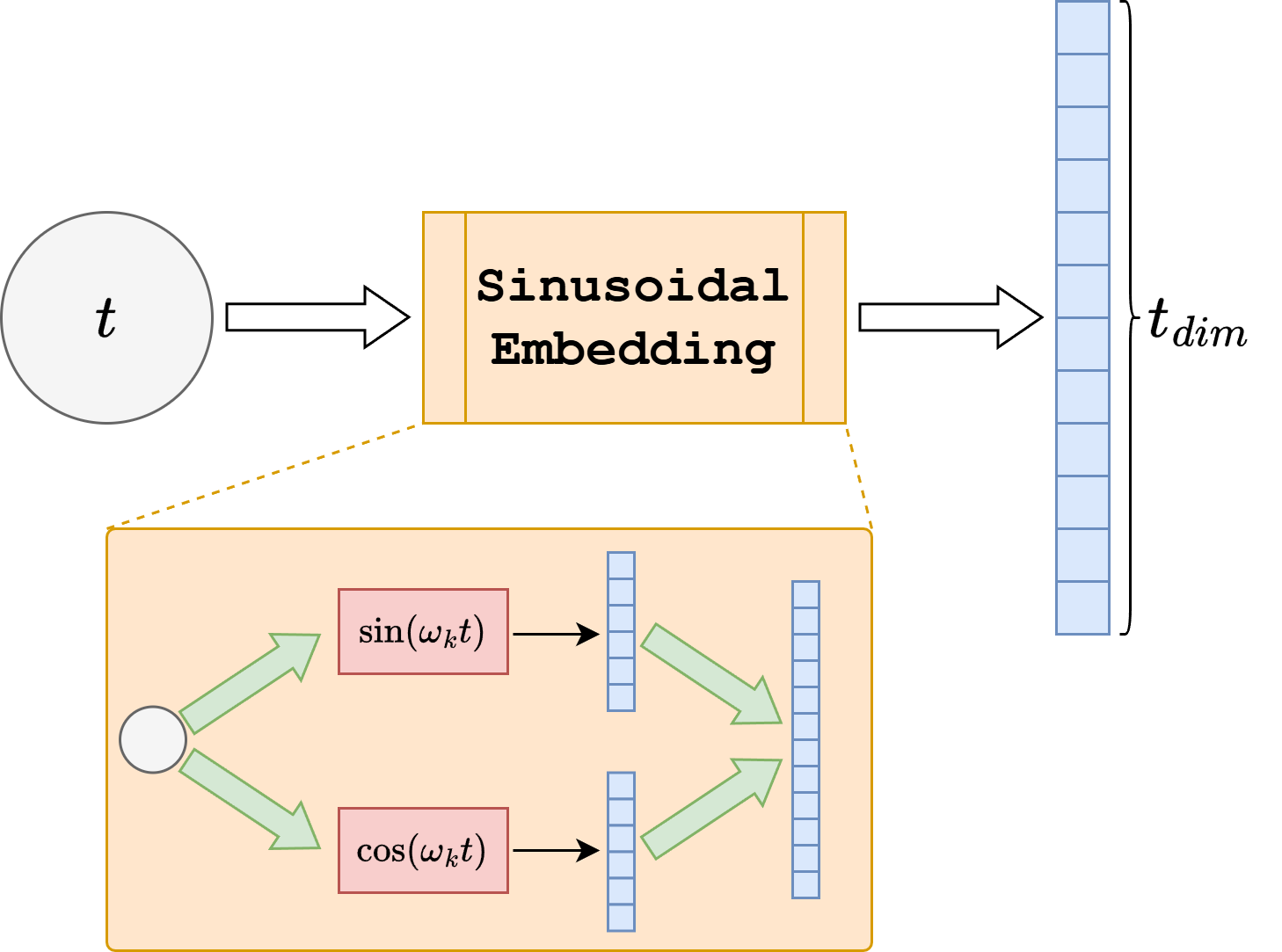
Fig. 39 A sinusoidal time embedding maps the scalar diffusion step into a multi-frequency vector representation. This lets the denoiser distinguish coarse and fine changes in the noise level while preserving smooth variation across time.#
Note
In diffusion code, time is not a cosmetic input. It tells the denoiser which perturbation regime it is looking at. A network without that context would be forced to solve many incompatible denoising problems with no indication of the current noise scale.
class SinusoidalTimeEmbedding(nn.Module):
    def __init__(self, dim):
        super().__init__()
        self.dim = dim

    def forward(self, t):
        half_dim = self.dim // 2
        factor = math.log(10000.0) / max(half_dim - 1, 1)
        frequencies = torch.exp(
            torch.arange(half_dim, device=t.device) * -factor
        )
        angles = t.float().unsqueeze(1) * frequencies.unsqueeze(0)
        embedding = torch.cat([angles.sin(), angles.cos()], dim=1)
        if self.dim % 2 == 1:
            embedding = F.pad(embedding, (0, 1))
        return embedding
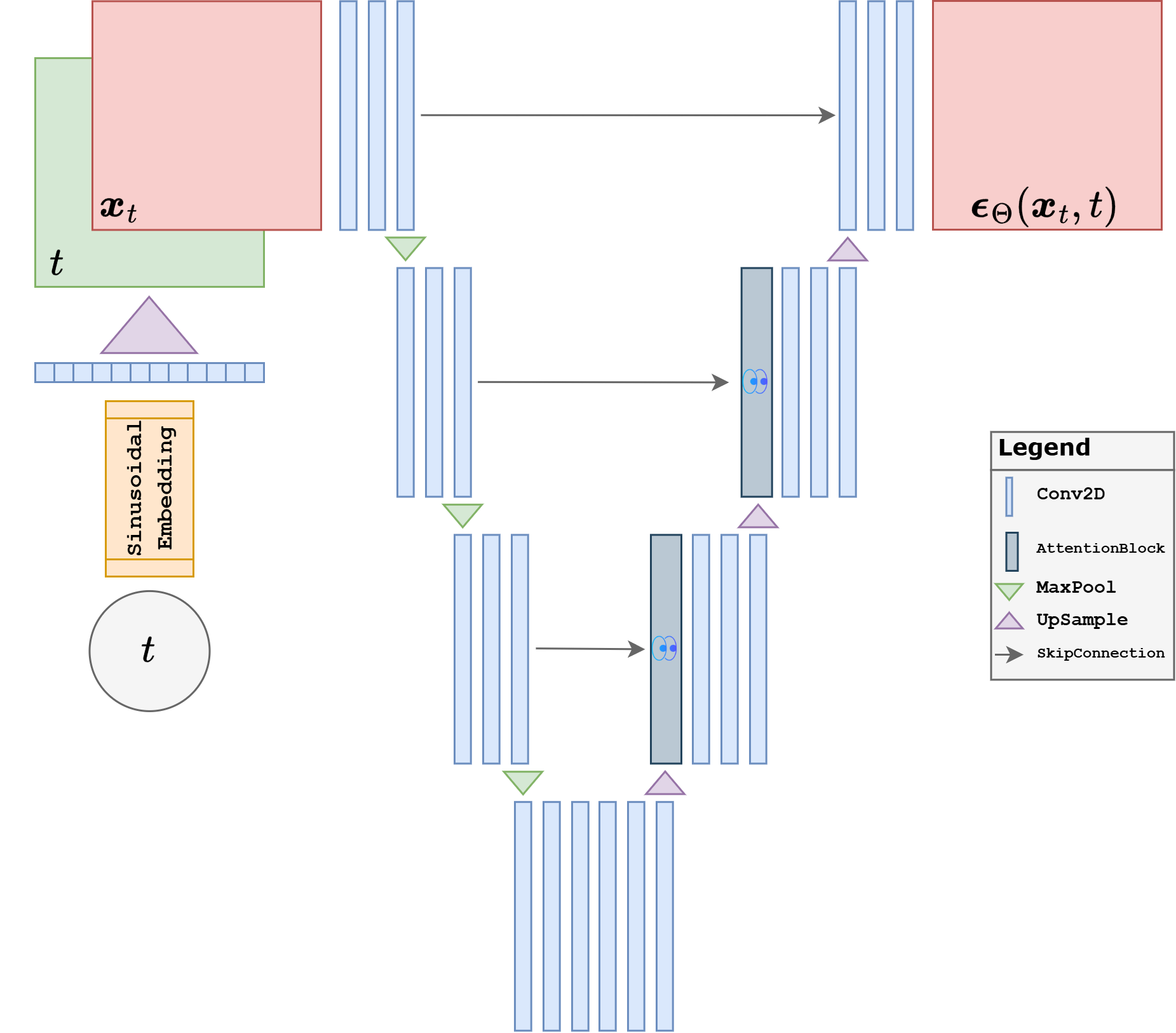
Fig. 40 The architecture used as a denoiser in diffusion models is typically a time-conditioned UNet.#
class ResidualBlock(nn.Module):
    def __init__(self, in_channels, out_channels, time_dim):
        super().__init__()
        self.conv1 = nn.Conv2d(in_channels, out_channels, kernel_size=3, padding=1)
        self.conv2 = nn.Conv2d(out_channels, out_channels, kernel_size=3, padding=1)
        self.time_mlp = nn.Linear(time_dim, out_channels)
        self.norm1 = nn.GroupNorm(8, out_channels)
        self.norm2 = nn.GroupNorm(8, out_channels)
        self.activation = nn.SiLU()
        self.residual = (
            nn.Conv2d(in_channels, out_channels, kernel_size=1)
            if in_channels != out_channels else nn.Identity()
        )

    def forward(self, x, t_emb):
        h = self.conv1(x)
        h = self.norm1(h)
        h = self.activation(h)

        # Broadcast the time embedding across spatial positions.
        time_term = self.time_mlp(t_emb).unsqueeze(-1).unsqueeze(-1)
        h = h + time_term

        h = self.conv2(h)
        h = self.norm2(h)
        h = self.activation(h)
        return h + self.residual(x)


class SmallUNet(nn.Module):
    def __init__(self, in_channels=1, base_channels=64, time_dim=128):
        super().__init__()
        self.time_embedding = nn.Sequential(
            SinusoidalTimeEmbedding(time_dim),
            nn.Linear(time_dim, time_dim),
            nn.SiLU(),
            nn.Linear(time_dim, time_dim),
        )

        self.input_conv = nn.Conv2d(in_channels, base_channels, kernel_size=3, padding=1)

        self.down1 = ResidualBlock(base_channels, base_channels, time_dim)
        self.downsample1 = nn.Conv2d(base_channels, base_channels * 2, kernel_size=4, stride=2, padding=1)
        self.down2 = ResidualBlock(base_channels * 2, base_channels * 2, time_dim)
        self.downsample2 = nn.Conv2d(base_channels * 2, base_channels * 4, kernel_size=4, stride=2, padding=1)
        self.down3 = ResidualBlock(base_channels * 4, base_channels * 4, time_dim)

        self.mid = ResidualBlock(base_channels * 4, base_channels * 4, time_dim)

        self.upsample2 = nn.ConvTranspose2d(base_channels * 4, base_channels * 2, kernel_size=4, stride=2, padding=1)
        self.up2 = ResidualBlock(base_channels * 4, base_channels * 2, time_dim)
        self.upsample1 = nn.ConvTranspose2d(base_channels * 2, base_channels, kernel_size=4, stride=2, padding=1)
        self.up1 = ResidualBlock(base_channels * 2, base_channels, time_dim)
        self.output_conv = nn.Conv2d(base_channels, in_channels, kernel_size=1)

    def forward(self, x, t):
        t_emb = self.time_embedding(t)

        # Save an early feature map so the decoder can recover detail later.
        x0 = self.input_conv(x)
        x1 = self.down1(x0, t_emb)
        x2 = self.downsample1(x1)
        x2 = self.down2(x2, t_emb)
        x3 = self.downsample2(x2)
        x3 = self.down3(x3, t_emb)

        x_mid = self.mid(x3, t_emb)

        x_up = self.upsample2(x_mid)
        x_up = torch.cat([x_up, x2], dim=1)
        x_up = self.up2(x_up, t_emb)
        x_up = self.upsample1(x_up)
        # Skip connection joins coarse semantics with finer spatial detail.
        x_up = torch.cat([x_up, x1], dim=1)
        x_up = self.up1(x_up, t_emb)
        return self.output_conv(x_up)


model = SmallUNet(in_channels=channels, base_channels=base_channels, time_dim=time_dim).to(device)
optimizer = torch.optim.Adam(model.parameters(), lr=lr)
Noise Prediction, Training, and the Meaning of the Loss#
The training target is the noise tensor itself. This is one of the most elegant aspects of DDPMs: a variational derivation over a long latent chain turns into an ordinary regression loss once the Gaussian forward process is chosen carefully. The model does not directly predict a clean image and it does not compete against a critic. It learns a local inverse problem indexed by time.
def diffusion_loss(model, x0, t):
    # Sample the corruption explicitly so the target noise is known.
    noise = torch.randn_like(x0)
    xt = q_sample(x0, t, noise)
    predicted_noise = model(xt, t)
    return F.mse_loss(predicted_noise, noise)
history = []

for epoch in tqdm(range(epochs), desc="Diffusion epochs"):
    model.train()
    running_loss = 0.0

    for x0, _ in tqdm(train_loader, desc="train", leave=False):
        x0 = x0.to(device)
        # Every image is trained at a randomly chosen noise level.
        t = torch.randint(0, timesteps, (x0.size(0),), device=device).long()

        optimizer.zero_grad()
        loss = diffusion_loss(model, x0, t)
        loss.backward()
        optimizer.step()

        running_loss += loss.item()

    epoch_loss = running_loss / len(train_loader)
    history.append(epoch_loss)
    print(f"Epoch {epoch + 1:02d} | loss: {epoch_loss:.6f}")


torch.save(model.state_dict(), ddpm_checkpoint_path)
print(f"Saved DDPM weights to {ddpm_checkpoint_path}")
Epoch 01 | loss: 0.135660
Epoch 02 | loss: 0.086285
Epoch 03 | loss: 0.080748
Epoch 04 | loss: 0.077359
Epoch 05 | loss: 0.074461
Epoch 06 | loss: 0.073934
Epoch 07 | loss: 0.072131
Epoch 08 | loss: 0.071382
Epoch 09 | loss: 0.069946
Epoch 10 | loss: 0.070485
Epoch 11 | loss: 0.069261
Epoch 12 | loss: 0.068826
Epoch 13 | loss: 0.068668
Epoch 14 | loss: 0.068250
Epoch 15 | loss: 0.067518
Epoch 16 | loss: 0.067611
Epoch 17 | loss: 0.067196
Epoch 18 | loss: 0.066250
Epoch 19 | loss: 0.066358
Epoch 20 | loss: 0.066262
Epoch 21 | loss: 0.066453
Epoch 22 | loss: 0.065976
Epoch 23 | loss: 0.065969
Epoch 24 | loss: 0.066058
Epoch 25 | loss: 0.065313
Epoch 26 | loss: 0.065062
Epoch 27 | loss: 0.064930
Epoch 28 | loss: 0.064869
Epoch 29 | loss: 0.064782
Epoch 30 | loss: 0.064992
Epoch 31 | loss: 0.064510
Epoch 32 | loss: 0.065199
Epoch 33 | loss: 0.063692
Epoch 34 | loss: 0.064107
Epoch 35 | loss: 0.064412
Epoch 36 | loss: 0.063475
Epoch 37 | loss: 0.064027
Epoch 38 | loss: 0.063494
Epoch 39 | loss: 0.064076
Epoch 40 | loss: 0.063515
Epoch 41 | loss: 0.062986
Epoch 42 | loss: 0.063544
Epoch 43 | loss: 0.063568
Epoch 44 | loss: 0.063168
Epoch 45 | loss: 0.063771
Epoch 46 | loss: 0.062650
Epoch 47 | loss: 0.063452
Epoch 48 | loss: 0.063447
Epoch 49 | loss: 0.062977
Epoch 50 | loss: 0.062572
Epoch 51 | loss: 0.062791
Epoch 52 | loss: 0.063233
Epoch 53 | loss: 0.062735
Epoch 54 | loss: 0.062655
Epoch 55 | loss: 0.061825
Epoch 56 | loss: 0.062399
Epoch 57 | loss: 0.062595
Epoch 58 | loss: 0.062476
Epoch 59 | loss: 0.062633
Epoch 60 | loss: 0.062617
Epoch 61 | loss: 0.062218
Epoch 62 | loss: 0.062148
Epoch 63 | loss: 0.062706
Epoch 64 | loss: 0.062336
Epoch 65 | loss: 0.062411
Epoch 66 | loss: 0.062665
Epoch 67 | loss: 0.061446
Epoch 68 | loss: 0.061728
Epoch 69 | loss: 0.062178
Epoch 70 | loss: 0.062340
Epoch 71 | loss: 0.062342
Epoch 72 | loss: 0.062110
Epoch 73 | loss: 0.061730
Epoch 74 | loss: 0.062061
Epoch 75 | loss: 0.061806
Epoch 76 | loss: 0.061444
Epoch 77 | loss: 0.062179
Epoch 78 | loss: 0.061926
Epoch 79 | loss: 0.061655
Epoch 80 | loss: 0.061425
Epoch 81 | loss: 0.060877
Epoch 82 | loss: 0.061116
Epoch 83 | loss: 0.061371
Epoch 84 | loss: 0.061205
Epoch 85 | loss: 0.061986
Epoch 86 | loss: 0.061501
Epoch 87 | loss: 0.061623
Epoch 88 | loss: 0.061183
Epoch 89 | loss: 0.061016
Epoch 90 | loss: 0.061062
Epoch 91 | loss: 0.061159
Epoch 92 | loss: 0.061338
Epoch 93 | loss: 0.060406
Epoch 94 | loss: 0.060793
Epoch 95 | loss: 0.061304
Epoch 96 | loss: 0.061200
Epoch 97 | loss: 0.061607
Epoch 98 | loss: 0.061748
Epoch 99 | loss: 0.060350
Epoch 100 | loss: 0.060916
Saved DDPM weights to c:\Users\tivog\deep-generative-models\artifacts\ddpm_fashionmnist.pt
plt.figure(figsize=(7, 4))
plt.plot(history)
plt.xlabel("Epoch")
plt.ylabel("Noise prediction loss")
plt.tight_layout()
plt.show()
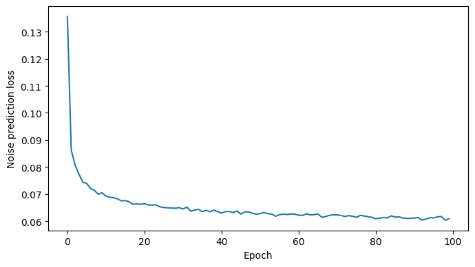
The resulting scalar loss is easier to interpret than a GAN loss because it is an honest regression objective, but it should still not be read in isolation. A lower MSE means the denoiser is learning something real, yet the visual quality of long reverse trajectories still depends on architecture, schedule, sampler, and training time.
DDPM Sampling, DDIM, and Quantitative Evaluation#
The reverse sampler is where the model becomes unmistakably generative. Each network evaluation only removes a small amount of noise, so synthesis requires many such evaluations chained together. This is also where the practical cost of diffusion appears most clearly.
The ancestral DDPM sampler is the most direct implementation of the learned reverse chain: estimate the clean image hidden in \(\boldsymbol{x}_t\), compute the reverse posterior mean, inject the correct amount of stochasticity, and continue. A deterministic DDIM sampler changes the trajectory while keeping the model fixed, which is one of the clearest examples of sampling engineering becoming as important as the learned denoiser itself.
@torch.no_grad()
def p_sample(model, x, t_scalar):
    t = torch.full((x.size(0),), t_scalar, device=device, dtype=torch.long)
    beta_t = extract(betas, t, x.shape)
    sqrt_one_minus_alpha_t = extract(sqrt_one_minus_alphas, t, x.shape)
    sqrt_recip_bar_alpha_t = extract(sqrt_recip_bar_alphas, t, x.shape)

    predicted_noise = model(x, t)
    x0_hat = (
        x - sqrt_one_minus_alpha_t * predicted_noise
    ) / extract(sqrt_alphas, t, x.shape)
    model_mean = sqrt_recip_bar_alpha_t * (
        x - beta_t * predicted_noise / sqrt_one_minus_alpha_t
    )

    if t_scalar == 0:
        return x0_hat.clamp(-1.0, 1.0)

    variance = extract(posterior_variance, t, x.shape)
    noise = torch.randn_like(x)
    return model_mean + torch.sqrt(variance) * noise


@torch.no_grad()
def sample_ddpm(model, n_samples=16, show_progress=True):
    model.eval()
    x = torch.randn(n_samples, channels, image_size, image_size, device=device)

    reverse_steps = reversed(range(timesteps))
    if show_progress:
        reverse_steps = tqdm(reverse_steps, total=timesteps, desc="ddpm sampling", leave=False)
    for t_scalar in reverse_steps:
        x = p_sample(model, x, t_scalar)

    x = x.clamp(-1, 1)
    x = 0.5 * (x + 1.0)
    return x.cpu()
The code above makes the DDPM logic explicit. The sampler predicts the noise, converts it into an estimate \(\hat{\boldsymbol{x}}_{0|t}\), uses that estimate to build the reverse mean, and then adds the stochastic term required by the Gaussian reverse conditional. This is the algorithmic form of “denoise a little, then move one step toward a cleaner image.”
@torch.no_grad()
def sample_ddim(model, n_samples=16, ddim_steps=50, eta=0.0, show_progress=True):
    model.eval()
    step_indices = torch.linspace(0, timesteps - 1, ddim_steps, device=device).long()
    x = torch.randn(n_samples, channels, image_size, image_size, device=device)

    iterator = reversed(range(ddim_steps))
    if show_progress:
        iterator = tqdm(iterator, total=ddim_steps, desc="ddim sampling", leave=False)

    for idx in iterator:
        t_scalar = step_indices[idx].item()
        t = torch.full((n_samples,), t_scalar, device=device, dtype=torch.long)
        predicted_noise = model(x, t)

        alpha_t = extract(alphas, t, x.shape)
        x0_hat = (
            x - extract(sqrt_one_minus_alphas, t, x.shape) * predicted_noise
        ) / extract(sqrt_alphas, t, x.shape)

        if idx == 0:
            x = x0_hat
            continue

        prev_t_scalar = step_indices[idx - 1].item()
        prev_t = torch.full((n_samples,), prev_t_scalar, device=device, dtype=torch.long)
        alpha_prev = extract(alphas, prev_t, x.shape)

        sigma_t = (
            eta
            * torch.sqrt((1 - alpha_prev) / (1 - alpha_t))
            * torch.sqrt(1 - alpha_t / alpha_prev)
        )
        direction = torch.sqrt(torch.clamp(1 - alpha_prev - sigma_t**2, min=0.0)) * predicted_noise
        noise = sigma_t * torch.randn_like(x) if eta > 0 else 0.0
        x = torch.sqrt(alpha_prev) * x0_hat + direction + noise

    x = x.clamp(-1, 1)
    x = 0.5 * (x + 1.0)
    return x.cpu()


ddpm_samples = sample_ddpm(model, n_samples=16)
ddim_samples = sample_ddim(model, n_samples=16, ddim_steps=50, eta=0.0)

plt.figure(figsize=(10, 5))
plt.subplot(1, 2, 1)
plt.imshow(utils.make_grid(ddpm_samples, nrow=4, pad_value=1.0).permute(1, 2, 0), cmap="gray")
plt.title("DDPM sampler")
plt.axis("off")

plt.subplot(1, 2, 2)
plt.imshow(utils.make_grid(ddim_samples, nrow=4, pad_value=1.0).permute(1, 2, 0), cmap="gray")
plt.title("DDIM sampler")
plt.axis("off")
plt.tight_layout()
plt.show()
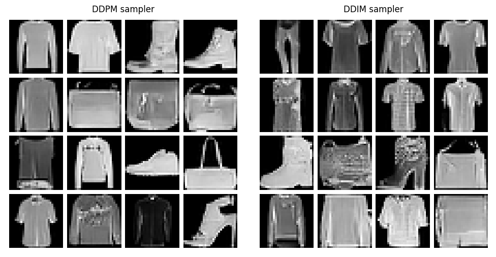
The step_indices array is the code-level manifestation of timestep skipping. A DDPM sampler uses every reverse step. A DDIM sampler may use only a subsequence of them, such as 50 steps instead of the full 300. The same denoiser is reused, but the numerical path through noise levels is coarser and often much faster.
Important
The practical identity of a diffusion system is model plus sampler, not only the denoiser. The same trained network can behave quite differently under ancestral DDPM updates and deterministic DDIM-style trajectories.
def prepare_for_inception_metrics(images):
    if images.size(1) == 1:
        images = images.repeat(1, 3, 1, 1)
    return images.clamp(0.0, 1.0)


@torch.no_grad()
def build_diffusion_metric_cache(real_loader, device, num_real=1000, metric_batch_size=32):
    fid = FrechetInceptionDistance(
        feature=2048,
        normalize=True,
        reset_real_features=False,
    ).set_dtype(torch.float64).to(device)
    kid = KernelInceptionDistance(
        feature=2048,
        subsets=10,
        subset_size=100,
        normalize=True,
        reset_real_features=False,
    ).to(device)

    seen_real = 0
    pbar = tqdm(total=num_real, desc="Diffusion real metrics", leave=False)
    for real_images, _ in real_loader:
        remaining = num_real - seen_real
        if remaining <= 0:
            break
        real_images = real_images[: min(metric_batch_size, remaining)].to(device)
        real_images = prepare_for_inception_metrics(0.5 * (real_images + 1.0))
        fid.update(real_images, real=True)
        kid.update(real_images, real=True)
        seen_real += real_images.size(0)
        pbar.update(real_images.size(0))
    pbar.close()
    return fid, kid


@torch.no_grad()
def evaluate_diffusion_sampler(sample_fn, base_fid, base_kid, device, num_fake=1000, metric_batch_size=32, desc="diffusion fake metrics"):
    fid = copy.deepcopy(base_fid)
    kid = copy.deepcopy(base_kid)

    generated = 0
    pbar = tqdm(total=num_fake, desc=desc, leave=False)
    while generated < num_fake:
        batch_n = min(metric_batch_size, num_fake - generated)
        fake_images = sample_fn(batch_n).to(device)
        fake_images = prepare_for_inception_metrics(fake_images)
        fid.update(fake_images, real=False)
        kid.update(fake_images, real=False)
        generated += batch_n
        pbar.update(batch_n)
    pbar.close()

    kid_mean, kid_std = kid.compute()
    return {
        "fid": fid.compute().item(),
        "kid_mean": kid_mean.item(),
        "kid_std": kid_std.item(),
    }


base_fid, base_kid = build_diffusion_metric_cache(
    train_loader,
    device,
    num_real=1000,
    metric_batch_size=32,
)

metric_scores = {
    "ddpm": evaluate_diffusion_sampler(
        lambda n: sample_ddpm(model, n_samples=n, show_progress=False),
        base_fid,
        base_kid,
        device,
        num_fake=1000,
        metric_batch_size=32,
        desc="DDPM fake metrics",
    ),
    "ddim": evaluate_diffusion_sampler(
        lambda n: sample_ddim(model, n_samples=n, ddim_steps=50, eta=0.0, show_progress=False),
        base_fid,
        base_kid,
        device,
        num_fake=1000,
        metric_batch_size=32,
        desc="DDIM fake metrics",
    ),
}
metric_scores
c:\Users\tivog\deep-generative-models\.venv\lib\site-packages\torchmetrics\utilities\prints.py:43: UserWarning: Metric `Kernel Inception Distance` will save all extracted features in buffer. For large datasets this may lead to large memory footprint.
  warnings.warn(*args, **kwargs)
{'ddpm': {'fid': 52.12181424960596,
  'kid_mean': 0.022715305909514427,
  'kid_std': 0.0032214955426752567},
 'ddim': {'fid': 72.84103285432505,
  'kid_mean': 0.04490206390619278,
  'kid_std': 0.003054284956306219}}
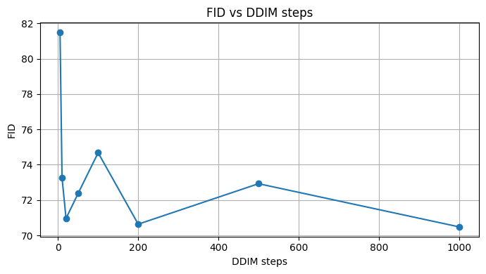
ddim_step_grid = [5, 10, 20, 50, 100, 200, 500, 1000]

ddim_steps = []
ddim_fids = []
ddim_kid_means = []
ddim_kid_stds = []

for steps in ddim_step_grid:
    scores = evaluate_diffusion_sampler(
        lambda n, steps=steps: sample_ddim(
            model,
            n_samples=n,
            ddim_steps=steps,
            eta=0.0,
            show_progress=False,
        ),
        base_fid,
        base_kid,
        device,
        num_fake=1000,
        metric_batch_size=32,
        desc=f"DDIM {steps} steps fake metrics",
    )

    ddim_steps.append(steps)
    ddim_fids.append(scores["fid"])
    ddim_kid_means.append(scores["kid_mean"])
    ddim_kid_stds.append(scores["kid_std"])

    print(
        f"DDIM steps={steps:>3} | "
        f"FID={scores['fid']:.4f} | "
        f"KID mean={scores['kid_mean']:.6f} | "
        f"KID std={scores['kid_std']:.6f}"
    )

# Plot FID as a function of DDIM steps.
plt.figure(figsize=(7, 4))
plt.plot(ddim_steps, ddim_fids, marker="o")
plt.xlabel("DDIM steps")
plt.ylabel("FID")
plt.title("FID vs DDIM steps")
plt.grid(True)
plt.tight_layout()
plt.show()
DDIM steps= 5 | FID=81.4924 | KID mean=0.051241 | KID std=0.006199
DDIM steps= 10 | FID=73.2568 | KID mean=0.045328 | KID std=0.008859
DDIM steps= 20 | FID=70.9603 | KID mean=0.046925 | KID std=0.007930
DDIM steps= 50 | FID=72.3716 | KID mean=0.044496 | KID std=0.008453
DDIM steps=100 | FID=74.6811 | KID mean=0.043048 | KID std=0.005816
DDIM steps=200 | FID=70.6352 | KID mean=0.043356 | KID std=0.008986
DDIM steps=500 | FID=72.9270 | KID mean=0.041166 | KID std=0.005933
DDIM steps=1000 | FID=70.4837 | KID mean=0.044855 | KID std=0.006326
Why Diffusion Models So Often Use a U-Net#
The denoiser in a diffusion model receives an image-like tensor at every time step and must return an image-like tensor of the same spatial size. This already explains why the U-Net became such a natural backbone. The model must read fine local evidence, aggregate information across scales, and then write back a spatially aligned correction. Skip connections are especially valuable here because denoising is not a task in which one wants to forget where structures are located. A noisy sleeve, shoe sole, or trouser edge is still roughly in the right place. The network benefits from preserving that spatial identity while gradually refining the content.
This multi-scale structure is also well matched to the actual reverse process. At large noise levels, the denoiser mostly needs coarse global cues: where the object is, what silhouette is emerging, and how mass should be distributed. At lower noise levels, the same network must correct smaller local defects such as texture, edge sharpness, and digit-like or fabric-like detail. A U-Net handles this progression well because it combines broad low-resolution context with high-resolution feature reuse.
Important
A diffusion denoiser is not only learning a probability model. It is also inheriting the inductive bias of its backbone. In practice, part of the visual behavior of diffusion models comes from the geometry of the U-Net itself.
The same architectural choice also creates a recognizable limitation. Even though a U-Net is multi-scale, its computation is still built from local convolutions, so the effective receptive field grows only gradually through depth and downsampling. This means that the denoiser is extremely good at restoring plausible local patches, but it can still struggle to enforce perfectly consistent global structure when many distant parts of the image must agree simultaneously. In high-resolution image synthesis, that weakness can manifest as duplicated details, broken symmetry, or the famous problem of generating the wrong number of fingers or other repeated anatomical parts.
From the viewpoint of receptive fields, the issue is intuitive. A local convolution sees a neighborhood, not the whole image at once. Global coherence must therefore emerge indirectly, after many layers have propagated information across space. If the model is underpowered, the training distribution is too broad, or the generation problem is especially compositional, local plausibility may win over global counting consistency. The image can look convincing in patches while still being wrong as an object.
A natural response is to replace or augment the U-Net with a Vision Transformer. Self-attention gives every token direct access to every other token, so long-range dependencies and object-level consistency can in principle be modeled more explicitly. This can help with precisely the kinds of failures that come from local receptive fields, including counting and global part-to-part agreement. The trade-off is that this global interaction is usually more expensive in memory and computation, and it often requires more careful optimization and larger-scale training to work well. For that reason, modern diffusion systems often mix the two ideas rather than treating them as mutually exclusive: convolutional structure remains attractive for efficiency and spatial bias, while attention layers are inserted where stronger global coordination is needed.