Variational Autoencoder Variants and Extensions

The vanilla VAE follows a clear principle: approximate maximum likelihood in a deep latent-variable model by optimizing the ELBO. This principle also exposes the main weaknesses of the model. The KL term may over-regularize the latent channel, some latent dimensions may become inactive, the aggregate posterior may fail to match the sampling prior, pixelwise likelihoods may encourage blurry averages, and unconditional generation gives little control over the type of sample produced.

VAE variants modify one of these ingredients while preserving the latent-variable structure. Some variants change the weight or schedule of the KL term. Some replace the continuous Gaussian bottleneck with a discrete codebook. Some condition the encoder and decoder on labels or other side information.

The discussion has two levels. The theoretical level describes which object changes: the objective, posterior family, prior, latent representation, or conditioning structure. The motivational level explains which vanilla-VAE limitation the change is meant to address. This mirrors the logic of the ELBO derivation: every architectural or objective modification should correspond to a precise modeling pressure.

How to read the variants

Each variant changes one pressure in the vanilla ELBO system: the strength of the KL term, the schedule of the information bottleneck, the type of latent representation, or the conditioning information available to the encoder and decoder.

Shared Setup

All variants below use the same FashionMNIST data pipeline and the same convolutional baseline components, so that comparisons remain meaningful. FID/KID is postponed to the end, so the real-data features only need to be accumulated once.

import copy
import torch
import torch.nn as nn
import torch.nn.functional as F
from pathlib import Path
from torch.utils.data import DataLoader, TensorDataset
from torchmetrics.image.fid import FrechetInceptionDistance
from torchmetrics.image.kid import KernelInceptionDistance
from torchvision import datasets, transforms, utils
from tqdm.auto import tqdm
import matplotlib.pyplot as plt

device = torch.device("cuda" if torch.cuda.is_available() else "cpu")
torch.manual_seed(7)
if device.type == "cuda":
    torch.cuda.manual_seed_all(7)
num_workers = 0
project_root = Path.cwd() if (Path.cwd() / "_config.yml").exists() else Path.cwd().parent
DATA_ROOT = project_root / "data"

# Settings
batch_size = 128
latent_dim = 32
base_channels = 32
lr = 2e-4
epochs = 60

transform = transforms.ToTensor()

train_dataset = datasets.FashionMNIST(
    root=DATA_ROOT,
    train=True,
    download=True,
    transform=transform,
)

test_dataset = datasets.FashionMNIST(
    root=DATA_ROOT,
    train=False,
    download=True,
    transform=transform,
)

train_loader = DataLoader(
    train_dataset,
    batch_size=batch_size,
    shuffle=True,
    num_workers=num_workers,
    pin_memory=(device.type == "cuda"),
)
test_loader = DataLoader(
    test_dataset,
    batch_size=batch_size,
    shuffle=False,
    num_workers=num_workers,
    pin_memory=(device.type == "cuda"),
)

class VAE(nn.Module):
    def __init__(self, latent_dim=32, base_channels=32):
        super().__init__()
        # 28x28 -> 14x14 -> 7x7.
        self.encoder = nn.Sequential(
            nn.Conv2d(1, base_channels, kernel_size=4, stride=2, padding=1),
            nn.BatchNorm2d(base_channels),
            nn.SiLU(),
            nn.Conv2d(base_channels, base_channels * 2, kernel_size=4, stride=2, padding=1),
            nn.BatchNorm2d(base_channels * 2),
            nn.SiLU(),
            nn.Conv2d(base_channels * 2, base_channels * 4, kernel_size=3, padding=1),
            nn.BatchNorm2d(base_channels * 4),
            nn.SiLU(),
            nn.Flatten(),
        )
        encoded_dim = base_channels * 4 * 7 * 7
        self.mu_head = nn.Linear(encoded_dim, latent_dim)
        self.logvar_head = nn.Linear(encoded_dim, latent_dim)

        self.decoder = nn.Sequential(
            nn.Linear(latent_dim, encoded_dim),
            nn.SiLU(),
            nn.Unflatten(1, (base_channels * 4, 7, 7)),
            nn.ConvTranspose2d(base_channels * 4, base_channels * 2, kernel_size=4, stride=2, padding=1),
            nn.BatchNorm2d(base_channels * 2),
            nn.SiLU(),
            nn.ConvTranspose2d(base_channels * 2, base_channels, kernel_size=4, stride=2, padding=1),
            nn.BatchNorm2d(base_channels),
            nn.SiLU(),
            nn.Conv2d(base_channels, 1, kernel_size=3, padding=1),
        )

    def encode(self, x):
        h = self.encoder(x)
        mu = self.mu_head(h)
        logvar = self.logvar_head(h)
        return mu, logvar

    def reparameterize(self, mu, logvar):
        # Sample through parameter-free noise so gradients can flow to mu/logvar.
        std = torch.exp(0.5 * logvar)
        eps = torch.randn_like(std)
        return mu + std * eps

    def decode(self, z):
        logits = self.decoder(z)
        return logits

    def forward(self, x):
        mu, logvar = self.encode(x)
        z = self.reparameterize(mu, logvar)
        logits = self.decode(z)
        return logits, mu, logvar


model = VAE(latent_dim=latent_dim, base_channels=base_channels).to(device)
optimizer = torch.optim.Adam(model.parameters(), lr=lr)

@torch.no_grad()
def show_reconstructions(model, loader, device, n=8):
    model.eval()
    x, _ = next(iter(loader))
    x = x[:n].to(device)
    logits, _, _ = model(x)
    # Sigmoid is only for visualization; training used logits directly.
    recon = torch.sigmoid(logits).view(-1, 1, 28, 28)

    grid = torch.cat([x.cpu(), recon.cpu()], dim=0)
    image = utils.make_grid(grid, nrow=n, pad_value=1.0)
    plt.figure(figsize=(1.5 * n, 3.0))
    plt.imshow(image.permute(1, 2, 0), cmap="gray")
    plt.axis("off")
    plt.show()


@torch.no_grad()
def show_samples(model, device, n=16):
    model.eval()
    z = torch.randn(n, latent_dim, device=device)
    logits = model.decode(z)
    samples = torch.sigmoid(logits).view(-1, 1, 28, 28).cpu()
    image = utils.make_grid(samples, nrow=4, pad_value=1.0)
    plt.figure(figsize=(6, 6))
    plt.imshow(image.permute(1, 2, 0), cmap="gray")
    plt.axis("off")
    plt.show()

@torch.no_grad()
def interpolate(model, loader, device, steps=8):
    model.eval()
    x, _ = next(iter(loader))
    x0 = x[0:1].to(device)
    x1 = x[1:2].to(device)

    # Interpolate between posterior means to visualize latent geometry.
    mu0, _ = model.encode(x0)
    mu1, _ = model.encode(x1)

    alphas = torch.linspace(0, 1, steps, device=device).view(-1, 1)
    z = (1 - alphas) * mu0 + alphas * mu1
    logits = model.decode(z)
    images = torch.sigmoid(logits).view(-1, 1, 28, 28).cpu()

    grid = utils.make_grid(images, nrow=steps, pad_value=1.0)
    plt.figure(figsize=(1.7 * steps, 2.5))
    plt.imshow(grid.permute(1, 2, 0), cmap="gray")
    plt.axis("off")
    plt.show()

Controlling Information Flow: Beta-VAE, KL Annealing, and Free Bits

The first family of VAE variants does not change the architecture in a dramatic way. It changes the pressure exerted by the objective on the latent channel. This is a good starting point because many practical VAE failures are not caused by an encoder or decoder that is obviously too small. They are caused by an objective that asks the model to satisfy two competing goals at the same time: reconstruct the data accurately and keep the approximate posterior close to a simple prior.

For a vanilla VAE, the objective minimized during training is the negative ELBO,

\[ \mathcal{L}_{VAE}(\boldsymbol{x}) = \mathbb{E}_{q_\phi(\boldsymbol{z}|\boldsymbol{x})} \left[-\log p_\theta(\boldsymbol{x}|\boldsymbol{z})\right] + D_{KL}\left(q_\phi(\boldsymbol{z}|\boldsymbol{x}) \| p(\boldsymbol{z})\right). \]

The first term is a distortion term: it measures how well the latent code reconstructs the input. The second term is a rate term: it measures how much information the encoder is allowed to transmit through the latent variable, relative to the prior. This terminology is useful because it makes the main tradeoff explicit. A model that uses a large rate can reconstruct well, but the posterior may become difficult to sample from using the simple prior. A model that uses a very small rate is easy to sample from, but the decoder receives little information about the input.

beta-VAE [HMP+17] modifies this tradeoff by introducing a scalar multiplier:

\[ \mathcal{L}_{\beta\text{-}VAE}(\boldsymbol{x}) = \mathbb{E}_{q_\phi(\boldsymbol{z}|\boldsymbol{x})} \left[-\log p_\theta(\boldsymbol{x}|\boldsymbol{z})\right] + \beta\, D_{KL}\left(q_\phi(\boldsymbol{z}|\boldsymbol{x}) \| p(\boldsymbol{z})\right). \]

When \(\beta>1\), the model pays a larger price for using information in the latent code. This can encourage a more compact representation and, in some settings, more interpretable latent factors. However, it can also damage reconstruction quality and increase the risk of inactive dimensions. When \(\beta<1\), the model is allowed to use the latent variable more freely. Reconstructions often improve, but samples drawn from the prior can become worse because the aggregate posterior may drift farther from the prior. Therefore, beta is not a quality knob that can simply be increased. It is a rate-control knob.

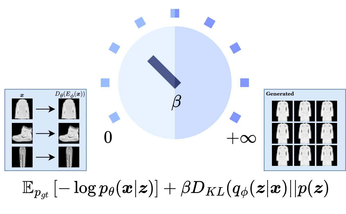
Fig. 20 The effect of \(\beta\) in \(\beta\)-VAE.

The theoretical perspective is that beta-VAE replaces likelihood maximization with a constrained or Lagrangian view of representation learning. Informally, one can read the objective as asking for small distortion subject to a limited information budget. Increasing beta tightens the budget. Decreasing beta relaxes it. The motivational perspective is simpler: the vanilla VAE has one fixed compromise between reconstruction and regularization, but different datasets and decoders need different compromises. beta-VAE gives us a way to move that compromise deliberately.

The limitation is that a fixed value of beta applies the same pressure throughout training. Early in training, the decoder and encoder do not yet know how to communicate. If the KL term is too strong at this stage, the easiest solution is to make the posterior close to the prior for every input. Once this happens, the decoder learns to work without the latent code, and the encoder may never recover. This is one route to posterior collapse.

In implementation terms, beta is the cleanest control knob in the VAE family. It does not change the latent-variable model or the encoder architecture. It changes only the relative strength of the KL term. The loss below therefore makes the rate-distortion interpretation visible in code.

Rate and distortion

Increasing \(\beta\) usually improves latent regularity at the cost of reconstruction detail. Decreasing \(\beta\) usually improves reconstruction at the cost of prior-sampling reliability.

def kl_per_sample(mu, logvar):
    # Keep the per-sample KL so we can reweight or threshold it flexibly.
    return -0.5 * torch.sum(1 + logvar - mu.pow(2) - logvar.exp(), dim=1)


def beta_vae_loss(x, logits, mu, logvar, beta=1.0, free_bits=0.0):
    reconstruction = F.binary_cross_entropy_with_logits(
        logits,
        x,
        reduction="sum",
    )
    kl_values = kl_per_sample(mu, logvar)
    if free_bits > 0.0:
        # Each sample is allowed to use a small amount of KL capacity for free.
        kl_values = torch.clamp(kl_values, min=free_bits)
    kl = kl_values.sum()
    loss = reconstruction + beta * kl
    return loss, reconstruction, kl


def linear_beta_schedule(epoch, total_epochs, start=0.0, stop=1.0, warmup_fraction=0.4):
    warmup_epochs = max(1, int(total_epochs * warmup_fraction))
    if epoch >= warmup_epochs:
        return stop
    progress = epoch / warmup_epochs
    return start + progress * (stop - start)

def train_beta_vae_epoch(model, loader, optimizer, device, beta=1.0):
    model.train()
    total_loss = 0.0
    total_kl = 0.0
    for x, _ in tqdm(loader, desc="beta-VAE train", leave=False):
        x = x.to(device)
        optimizer.zero_grad()
        logits, mu, logvar = model(x)
        loss, _, kl = beta_vae_loss(x, logits, mu, logvar, beta=beta)
        loss.backward()
        optimizer.step()
        total_loss += loss.item()
        total_kl += kl.item()
    n = len(loader.dataset)
    return {"loss": total_loss / n, "kl": total_kl / n}


@torch.no_grad()
def evaluate_beta_vae(model, loader, device, beta=1.0):
    model.eval()
    total_loss = 0.0
    total_kl = 0.0
    for x, _ in loader:
        x = x.to(device)
        logits, mu, logvar = model(x)
        loss, _, kl = beta_vae_loss(x, logits, mu, logvar, beta=beta)
        total_loss += loss.item()
        total_kl += kl.item()
    n = len(loader.dataset)
    return {"loss": total_loss / n, "kl": total_kl / n}


beta_model = VAE(latent_dim=latent_dim, base_channels=base_channels).to(device)
beta_optimizer = torch.optim.Adam(beta_model.parameters(), lr=lr)
beta_history = {"train_loss": [], "val_loss": [], "kl": []}
beta_epochs = 50
beta_value = 4.0

for epoch in tqdm(range(beta_epochs), desc="beta-VAE epochs"):
    train_stats = train_beta_vae_epoch(beta_model, train_loader, beta_optimizer, device, beta=beta_value)
    val_stats = evaluate_beta_vae(beta_model, test_loader, device, beta=beta_value)
    beta_history["train_loss"].append(train_stats["loss"])
    beta_history["val_loss"].append(val_stats["loss"])
    beta_history["kl"].append(train_stats["kl"])
    print(
        f"Epoch {epoch + 1:02d} | beta={beta_value:.1f} | "
        f"train loss: {train_stats['loss']:.4f} | "
        f"val loss: {val_stats['loss']:.4f} | "
        f"KL: {train_stats['kl']:.4f}"
    )

Epoch 01 | beta=4.0 | train loss: 325.6506 | val loss: 292.6421 | KL: 6.8962

Epoch 02 | beta=4.0 | train loss: 286.8193 | val loss: 284.9199 | KL: 7.1615

Epoch 03 | beta=4.0 | train loss: 282.1822 | val loss: 281.7744 | KL: 7.1447

Epoch 04 | beta=4.0 | train loss: 279.8793 | val loss: 280.4502 | KL: 7.1589

Epoch 05 | beta=4.0 | train loss: 278.4796 | val loss: 278.9888 | KL: 7.1442

Epoch 06 | beta=4.0 | train loss: 277.2528 | val loss: 278.4609 | KL: 7.1314

Epoch 07 | beta=4.0 | train loss: 276.3851 | val loss: 277.2093 | KL: 7.1493

Epoch 08 | beta=4.0 | train loss: 275.7498 | val loss: 276.7020 | KL: 7.1358

Epoch 09 | beta=4.0 | train loss: 275.2038 | val loss: 276.0955 | KL: 7.1390

Epoch 10 | beta=4.0 | train loss: 274.6195 | val loss: 275.4439 | KL: 7.1239

Epoch 11 | beta=4.0 | train loss: 274.0574 | val loss: 275.3861 | KL: 7.1219

Epoch 12 | beta=4.0 | train loss: 273.6356 | val loss: 274.7167 | KL: 7.1247

Epoch 13 | beta=4.0 | train loss: 273.2184 | val loss: 274.4480 | KL: 7.1160

Epoch 14 | beta=4.0 | train loss: 272.8187 | val loss: 274.9395 | KL: 7.1037

Epoch 15 | beta=4.0 | train loss: 272.6882 | val loss: 274.0135 | KL: 7.1298

Epoch 16 | beta=4.0 | train loss: 272.2482 | val loss: 273.6034 | KL: 7.1215

Epoch 17 | beta=4.0 | train loss: 272.0446 | val loss: 273.4072 | KL: 7.1382

Epoch 18 | beta=4.0 | train loss: 271.8151 | val loss: 272.9650 | KL: 7.1451

Epoch 19 | beta=4.0 | train loss: 271.4919 | val loss: 273.0315 | KL: 7.1218

Epoch 20 | beta=4.0 | train loss: 271.4045 | val loss: 272.6747 | KL: 7.1421

Epoch 21 | beta=4.0 | train loss: 271.1198 | val loss: 272.4825 | KL: 7.1335

Epoch 22 | beta=4.0 | train loss: 270.9852 | val loss: 272.2881 | KL: 7.1293

Epoch 23 | beta=4.0 | train loss: 270.7618 | val loss: 272.1179 | KL: 7.1342

Epoch 24 | beta=4.0 | train loss: 270.6377 | val loss: 272.2479 | KL: 7.1504

Epoch 25 | beta=4.0 | train loss: 270.4983 | val loss: 272.3169 | KL: 7.1569

Epoch 26 | beta=4.0 | train loss: 270.3835 | val loss: 271.5416 | KL: 7.1545

Epoch 27 | beta=4.0 | train loss: 270.1452 | val loss: 272.0160 | KL: 7.1433

Epoch 28 | beta=4.0 | train loss: 270.0638 | val loss: 271.2311 | KL: 7.1464

Epoch 29 | beta=4.0 | train loss: 269.9422 | val loss: 271.1200 | KL: 7.1484

Epoch 30 | beta=4.0 | train loss: 269.9100 | val loss: 271.1127 | KL: 7.1536

Epoch 31 | beta=4.0 | train loss: 269.7316 | val loss: 271.1946 | KL: 7.1574

Epoch 32 | beta=4.0 | train loss: 269.6192 | val loss: 271.0486 | KL: 7.1596

Epoch 33 | beta=4.0 | train loss: 269.5483 | val loss: 270.6967 | KL: 7.1508

Epoch 34 | beta=4.0 | train loss: 269.3049 | val loss: 270.8625 | KL: 7.1483

Epoch 35 | beta=4.0 | train loss: 269.3250 | val loss: 270.5647 | KL: 7.1590

Epoch 36 | beta=4.0 | train loss: 269.2298 | val loss: 270.5957 | KL: 7.1661

Epoch 37 | beta=4.0 | train loss: 269.0788 | val loss: 270.1812 | KL: 7.1556

Epoch 38 | beta=4.0 | train loss: 268.9993 | val loss: 270.3317 | KL: 7.1554

Epoch 39 | beta=4.0 | train loss: 268.9553 | val loss: 270.7439 | KL: 7.1651

Epoch 40 | beta=4.0 | train loss: 268.9308 | val loss: 270.3053 | KL: 7.1738

Epoch 41 | beta=4.0 | train loss: 268.7867 | val loss: 270.2550 | KL: 7.1778

Epoch 42 | beta=4.0 | train loss: 268.7642 | val loss: 270.6089 | KL: 7.1753

Epoch 43 | beta=4.0 | train loss: 268.6302 | val loss: 269.9276 | KL: 7.1769

Epoch 44 | beta=4.0 | train loss: 268.5707 | val loss: 270.0085 | KL: 7.1756

Epoch 45 | beta=4.0 | train loss: 268.5426 | val loss: 270.2158 | KL: 7.1739

Epoch 46 | beta=4.0 | train loss: 268.4228 | val loss: 270.0582 | KL: 7.1718

Epoch 47 | beta=4.0 | train loss: 268.4645 | val loss: 269.8492 | KL: 7.1885

Epoch 48 | beta=4.0 | train loss: 268.3688 | val loss: 269.9342 | KL: 7.1884

Epoch 49 | beta=4.0 | train loss: 268.2670 | val loss: 269.5371 | KL: 7.1935

Epoch 50 | beta=4.0 | train loss: 268.2067 | val loss: 269.9617 | KL: 7.1944

A useful qualitative comparison is obtained by placing this run next to the vanilla VAE. Larger beta values often produce a more organized latent space but softer reconstructions. Smaller beta values often improve reconstruction while making prior sampling less reliable. The visible samples are therefore an empirical picture of the same rate-distortion tradeoff described by the objective.

show_reconstructions(beta_model, test_loader, device)
show_samples(beta_model, device)
interpolate(beta_model, test_loader, device)

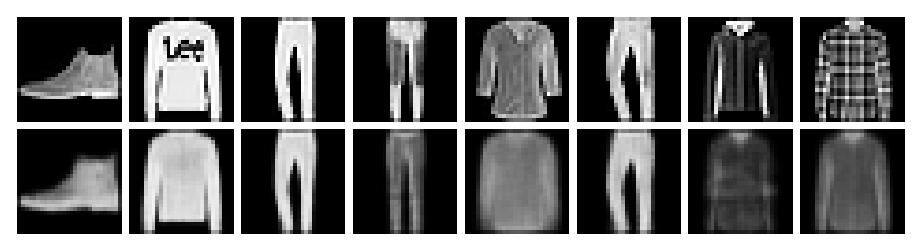
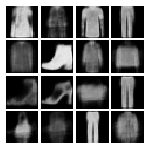
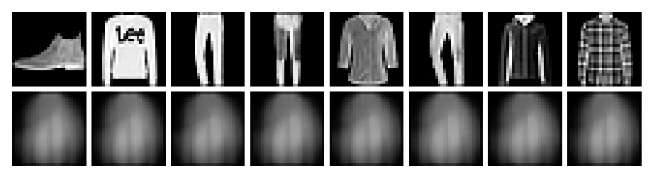
If the value of \(\beta\) is set too high, the \(D_{KL}\) term dominates and \(q_\phi(\boldsymbol{z} | \boldsymbol{x})\) becomes uninformative, causing mode collapse.

beta_collapse_model = VAE(latent_dim=latent_dim, base_channels=base_channels).to(device)
beta_optimizer = torch.optim.Adam(beta_collapse_model.parameters(), lr=lr)
beta_collapse_history = {"train_loss": [], "val_loss": [], "kl": []}
beta_epochs = 50
beta_value = 100.0

for epoch in range(beta_epochs):
    train_stats = train_beta_vae_epoch(beta_collapse_model, train_loader, beta_optimizer, device, beta=beta_value)
    val_stats = evaluate_beta_vae(beta_collapse_model, test_loader, device, beta=beta_value)
    beta_collapse_history["train_loss"].append(train_stats["loss"])
    beta_collapse_history["val_loss"].append(val_stats["loss"])
    beta_collapse_history["kl"].append(train_stats["kl"])
    print(
        f"Epoch {epoch + 1:02d} | beta={beta_value:.1f} | "
        f"train loss: {train_stats['loss']:.4f} | "
        f"val loss: {val_stats['loss']:.4f} | "
        f"KL: {train_stats['kl']:.4f}"
    )

show_reconstructions(beta_collapse_model, test_loader, device)
show_samples(beta_collapse_model, device)
interpolate(beta_collapse_model, test_loader, device)

Epoch 01 | beta=100.0 | train loss: 408.9631 | val loss: 388.7563 | KL: 0.0936

Epoch 02 | beta=100.0 | train loss: 387.0263 | val loss: 387.5785 | KL: 0.0155

Epoch 03 | beta=100.0 | train loss: 386.1280 | val loss: 386.8369 | KL: 0.0112

Epoch 04 | beta=100.0 | train loss: 385.7847 | val loss: 386.3877 | KL: 0.0113

Epoch 05 | beta=100.0 | train loss: 385.5996 | val loss: 386.2267 | KL: 0.0091

Epoch 06 | beta=100.0 | train loss: 385.4597 | val loss: 386.7706 | KL: 0.0081

Epoch 07 | beta=100.0 | train loss: 385.3594 | val loss: 385.8701 | KL: 0.0081

Epoch 08 | beta=100.0 | train loss: 385.3668 | val loss: 386.1426 | KL: 0.0092

Epoch 09 | beta=100.0 | train loss: 385.3468 | val loss: 385.9713 | KL: 0.0073

Epoch 10 | beta=100.0 | train loss: 385.1523 | val loss: 386.2815 | KL: 0.0058

Epoch 11 | beta=100.0 | train loss: 385.0837 | val loss: 385.9519 | KL: 0.0064

Epoch 12 | beta=100.0 | train loss: 385.0521 | val loss: 386.0125 | KL: 0.0074

Epoch 13 | beta=100.0 | train loss: 385.0704 | val loss: 385.6226 | KL: 0.0074

Epoch 14 | beta=100.0 | train loss: 385.0038 | val loss: 385.7704 | KL: 0.0055

Epoch 15 | beta=100.0 | train loss: 384.9677 | val loss: 385.6601 | KL: 0.0062

Epoch 16 | beta=100.0 | train loss: 384.9214 | val loss: 385.4832 | KL: 0.0048

Epoch 17 | beta=100.0 | train loss: 384.8163 | val loss: 385.5935 | KL: 0.0039

Epoch 18 | beta=100.0 | train loss: 384.8450 | val loss: 385.5045 | KL: 0.0041

Epoch 19 | beta=100.0 | train loss: 384.8412 | val loss: 385.3939 | KL: 0.0035

Epoch 20 | beta=100.0 | train loss: 384.7763 | val loss: 385.4679 | KL: 0.0038

Epoch 21 | beta=100.0 | train loss: 384.7466 | val loss: 385.4655 | KL: 0.0041

Epoch 22 | beta=100.0 | train loss: 384.7298 | val loss: 385.5660 | KL: 0.0043

Epoch 23 | beta=100.0 | train loss: 384.7532 | val loss: 385.2891 | KL: 0.0033

Epoch 24 | beta=100.0 | train loss: 384.7142 | val loss: 385.2996 | KL: 0.0030

Epoch 25 | beta=100.0 | train loss: 384.6909 | val loss: 385.3590 | KL: 0.0029

Epoch 26 | beta=100.0 | train loss: 384.6657 | val loss: 385.3076 | KL: 0.0031

Epoch 27 | beta=100.0 | train loss: 384.6681 | val loss: 385.4229 | KL: 0.0028

Epoch 28 | beta=100.0 | train loss: 384.6710 | val loss: 385.3543 | KL: 0.0023

Epoch 29 | beta=100.0 | train loss: 384.6265 | val loss: 385.4636 | KL: 0.0025

Epoch 30 | beta=100.0 | train loss: 384.6489 | val loss: 385.2829 | KL: 0.0028

Epoch 31 | beta=100.0 | train loss: 384.6406 | val loss: 385.2762 | KL: 0.0025

Epoch 32 | beta=100.0 | train loss: 384.6015 | val loss: 385.4098 | KL: 0.0026

Epoch 33 | beta=100.0 | train loss: 384.6073 | val loss: 385.1796 | KL: 0.0028

Epoch 34 | beta=100.0 | train loss: 384.6295 | val loss: 385.3289 | KL: 0.0024

Epoch 35 | beta=100.0 | train loss: 384.6055 | val loss: 385.2529 | KL: 0.0020

Epoch 36 | beta=100.0 | train loss: 384.6006 | val loss: 385.2451 | KL: 0.0020

Epoch 37 | beta=100.0 | train loss: 384.5830 | val loss: 385.0939 | KL: 0.0024

Epoch 38 | beta=100.0 | train loss: 384.5599 | val loss: 385.2089 | KL: 0.0025

Epoch 39 | beta=100.0 | train loss: 384.5766 | val loss: 385.4060 | KL: 0.0028

Epoch 40 | beta=100.0 | train loss: 384.5946 | val loss: 385.5284 | KL: 0.0022

Epoch 41 | beta=100.0 | train loss: 384.5498 | val loss: 385.1983 | KL: 0.0024

Epoch 42 | beta=100.0 | train loss: 384.5912 | val loss: 385.1728 | KL: 0.0030

Epoch 43 | beta=100.0 | train loss: 384.5370 | val loss: 385.1624 | KL: 0.0024

Epoch 44 | beta=100.0 | train loss: 384.5758 | val loss: 385.1117 | KL: 0.0021

Epoch 45 | beta=100.0 | train loss: 384.5883 | val loss: 385.2598 | KL: 0.0020

Epoch 46 | beta=100.0 | train loss: 384.5429 | val loss: 385.3633 | KL: 0.0017

Epoch 47 | beta=100.0 | train loss: 384.5302 | val loss: 385.3264 | KL: 0.0024

Epoch 48 | beta=100.0 | train loss: 384.5634 | val loss: 385.5393 | KL: 0.0023

Epoch 49 | beta=100.0 | train loss: 384.5199 | val loss: 385.2124 | KL: 0.0022

Epoch 50 | beta=100.0 | train loss: 384.5532 | val loss: 385.2287 | KL: 0.0021

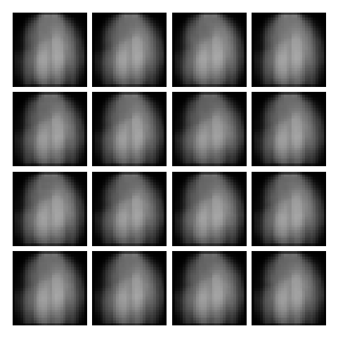
KL Annealing, Free Bits, and Posterior Collapse

KL annealing and free bits are two attempts to make the information budget dynamic rather than fixed. They are motivated by the observation that the most dangerous moment for posterior collapse is often the beginning of training. At that point, the decoder can reduce the reconstruction loss by learning broad regularities of the data, while the encoder is immediately penalized for transmitting information. If the optimizer discovers that ignoring \(\boldsymbol{z}\) is a stable solution, the latent channel can become inactive before it becomes useful.

KL annealing changes the training objective over time:

\[ \mathcal{L}_{anneal}(\boldsymbol{x},t) = \mathbb{E}_{q_\phi(\boldsymbol{z}|\boldsymbol{x})} \left[-\log p_\theta(\boldsymbol{x}|\boldsymbol{z})\right] + \beta(t) D_{KL}\left(q_\phi(\boldsymbol{z}|\boldsymbol{x}) \| p(\boldsymbol{z})\right), \]

where \(\beta(t)\) starts near zero and gradually increases toward its target value. The mechanism is simple but important. At the beginning, the model is encouraged to learn an informative autoencoding channel. Later, the KL pressure is increased so that the learned representation becomes compatible with the prior. In motivational terms, KL annealing first teaches the model to speak through the latent variable, and only later teaches it to speak economically.

Free bits attack the same problem from a different angle. Instead of globally reducing the KL weight, free bits define a minimum amount of information that the model can use without being penalized too aggressively. For a latent vector with coordinate-wise KL contributions, one common form is

\[ \mathcal{L}_{free}(\boldsymbol{x}) = \mathbb{E}_{q_\phi(\boldsymbol{z}|\boldsymbol{x})} \left[-\log p_\theta(\boldsymbol{x}|\boldsymbol{z})\right] + \sum_{\ell=1}^{L} \max\left(\lambda, D_{KL}\left(q_\phi(z_\ell|\boldsymbol{x}) \| p(z_\ell)\right)\right). \]

The constant \(\lambda\) is the number of free bits assigned to each latent component or group of components. Below this threshold, reducing the KL further does not improve the objective. This discourages the optimizer from spending effort on making already-small KL terms even smaller. In practical language, free bits tell the model: use at least a small amount of capacity before I start charging you for it.

The connection with dead latent dimensions is direct. For a diagonal Gaussian encoder,

\[ q_\phi(\boldsymbol{z}|\boldsymbol{x}) = \mathcal{N}\left( \boldsymbol{\mu}_\phi(\boldsymbol{x}), \operatorname{diag}(\boldsymbol{\sigma}^2_\phi(\boldsymbol{x})) \right), \]

a dimension is inactive when \(\mu_{\phi,\ell}(\boldsymbol{x}) \approx 0\) and \(\sigma_{\phi,\ell}(\boldsymbol{x}) \approx 1\) for almost all inputs. In that case,

\[ q_\phi(z_\ell|\boldsymbol{x}) \approx p(z_\ell), \]

so the coordinate carries almost no information about \(\boldsymbol{x}\). This is sometimes called a dead or collapsed latent dimension. The word collapsed does not mean that the numerical value is constant. It means that the posterior distribution for that coordinate is essentially the prior, so sampling that coordinate tells the decoder almost nothing about the input.

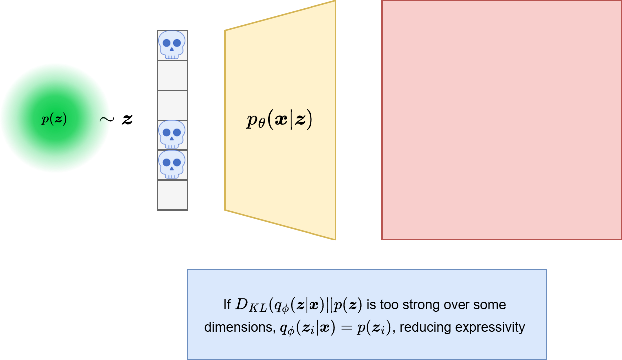
Fig. 21 The effect of collapsed latent dimensions.

KL annealing and free bits are not guaranteed cures. If the decoder is too powerful, if the latent dimensionality is badly chosen, or if the likelihood model rewards averaging, the latent channel can still be underused. But these methods make the optimization path less hostile to latent-variable usage. They are also cheap, which makes them important baselines: before introducing a new generative paradigm, one should first understand how far the original VAE can be improved by changing the objective.

annealed_model = VAE(latent_dim=latent_dim, base_channels=base_channels).to(device)
annealed_optimizer = torch.optim.Adam(annealed_model.parameters(), lr=lr)
annealed_history = {"train_loss": [], "val_loss": [], "beta": []}
annealed_epochs = 50
free_bits_value = 0.1

for epoch in tqdm(range(annealed_epochs), desc="annealed VAE epochs"):
    beta_t = linear_beta_schedule(epoch, annealed_epochs, start=0.0, stop=1.0, warmup_fraction=0.4)
    annealed_model.train()
    total_loss = 0.0
    for x, _ in tqdm(train_loader, desc="annealed train", leave=False):
        x = x.to(device)
        annealed_optimizer.zero_grad()
        logits, mu, logvar = annealed_model(x)
        loss, _, _ = beta_vae_loss(x, logits, mu, logvar, beta=beta_t, free_bits=free_bits_value)
        loss.backward()
        annealed_optimizer.step()
        total_loss += loss.item()
    annealed_history["train_loss"].append(total_loss / len(train_loader.dataset))
    annealed_history["beta"].append(beta_t)
    print(f"Epoch {epoch + 1:02d} | beta_t={beta_t:.2f} | train loss: {annealed_history['train_loss'][-1]:.4f}")

Epoch 01 | beta_t=0.00 | train loss: 265.2941

Epoch 02 | beta_t=0.05 | train loss: 223.2193

Epoch 03 | beta_t=0.10 | train loss: 221.9041

Epoch 04 | beta_t=0.15 | train loss: 222.8430

Epoch 05 | beta_t=0.20 | train loss: 224.2579

Epoch 06 | beta_t=0.25 | train loss: 225.7513

Epoch 07 | beta_t=0.30 | train loss: 227.2235

Epoch 08 | beta_t=0.35 | train loss: 228.6176

Epoch 09 | beta_t=0.40 | train loss: 229.9835

Epoch 10 | beta_t=0.45 | train loss: 231.1839

Epoch 11 | beta_t=0.50 | train loss: 232.3225

Epoch 12 | beta_t=0.55 | train loss: 233.4648

Epoch 13 | beta_t=0.60 | train loss: 234.5796

Epoch 14 | beta_t=0.65 | train loss: 235.5439

Epoch 15 | beta_t=0.70 | train loss: 236.5129

Epoch 16 | beta_t=0.75 | train loss: 237.4027

Epoch 17 | beta_t=0.80 | train loss: 238.2950

Epoch 18 | beta_t=0.85 | train loss: 239.1666

Epoch 19 | beta_t=0.90 | train loss: 239.9215

Epoch 20 | beta_t=0.95 | train loss: 240.7047

Epoch 21 | beta_t=1.00 | train loss: 241.4145

Epoch 22 | beta_t=1.00 | train loss: 241.1507

Epoch 23 | beta_t=1.00 | train loss: 240.8998

Epoch 24 | beta_t=1.00 | train loss: 240.6985

Epoch 25 | beta_t=1.00 | train loss: 240.4851

Epoch 26 | beta_t=1.00 | train loss: 240.2855

Epoch 27 | beta_t=1.00 | train loss: 240.1118

Epoch 28 | beta_t=1.00 | train loss: 239.9107

Epoch 29 | beta_t=1.00 | train loss: 239.7310

Epoch 30 | beta_t=1.00 | train loss: 239.5750

Epoch 31 | beta_t=1.00 | train loss: 239.3827

Epoch 32 | beta_t=1.00 | train loss: 239.2983

Epoch 33 | beta_t=1.00 | train loss: 239.0784

Epoch 34 | beta_t=1.00 | train loss: 239.0192

Epoch 35 | beta_t=1.00 | train loss: 238.9020

Epoch 36 | beta_t=1.00 | train loss: 238.7362

Epoch 37 | beta_t=1.00 | train loss: 238.6285

Epoch 38 | beta_t=1.00 | train loss: 238.5061

Epoch 39 | beta_t=1.00 | train loss: 238.4078

Epoch 40 | beta_t=1.00 | train loss: 238.3320

Epoch 41 | beta_t=1.00 | train loss: 238.2056

Epoch 42 | beta_t=1.00 | train loss: 238.1151

Epoch 43 | beta_t=1.00 | train loss: 238.0404

Epoch 44 | beta_t=1.00 | train loss: 237.9194

Epoch 45 | beta_t=1.00 | train loss: 237.8188

Epoch 46 | beta_t=1.00 | train loss: 237.7369

Epoch 47 | beta_t=1.00 | train loss: 237.6923

Epoch 48 | beta_t=1.00 | train loss: 237.5838

Epoch 49 | beta_t=1.00 | train loss: 237.6048

Epoch 50 | beta_t=1.00 | train loss: 237.4596

This experiment is conceptually different from the fixed-beta run. The question is no longer only how tight the final bottleneck should be. The question is how the bottleneck should be introduced during optimization. A schedule that starts gently and becomes stricter later can preserve latent usage while still ending with a structured latent space.

show_reconstructions(beta_model, test_loader, device)
show_samples(beta_model, device)
interpolate(beta_model, test_loader, device)

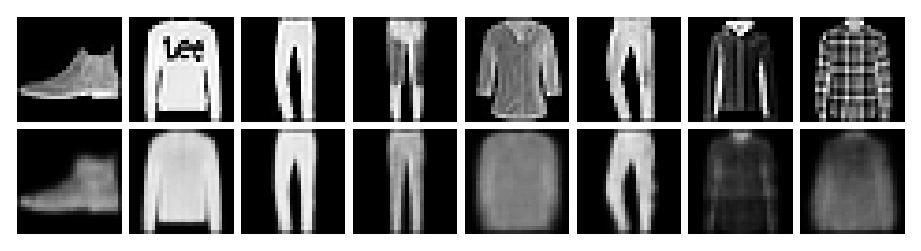
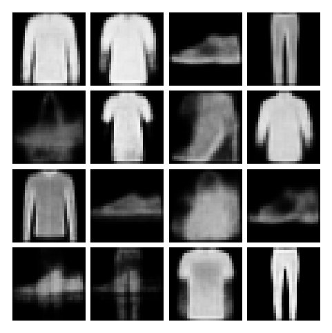
The scheduling function is important because a fixed beta=4 from the first iteration and a run that ends near beta=4 after a warm-up are not the same optimization problem. In the first case, the optimizer may shut down the latent channel before it ever becomes useful. In the second case, the model first learns to communicate through \(\boldsymbol{z}\) and only later tightens the information budget.

Taken together, beta-VAE, KL annealing, and **free bits** show that VAE design is not only about the existence of a latent variable. It is also about how much information is allowed to pass through the latent channel and when that information becomes expensive.

VQ-VAE and Discrete Latent Spaces

The second major branch of VAE variants changes something more radical than the information-control family. A beta-VAE, KL annealing, and free bits still keep the same basic object: an encoder produces the parameters of a continuous approximate posterior, usually a Gaussian distribution, and generation starts by sampling a continuous latent vector from a simple prior. A VQ-VAE, introduced in [vdOVK17], changes the type of latent representation itself. The encoder does not output the mean and variance of a Gaussian posterior. It outputs a spatial grid of vectors, and each vector is replaced by the closest element of a learned finite dictionary, usually called a codebook.

This change is motivated by a limitation that appears repeatedly in vanilla VAEs. The decoder is trained through a reconstruction term, while the encoder is regularized toward a simple prior. If the decoder is expressive and the KL pressure is strong, the model can learn to ignore part of the latent channel. If the latent channel is used only weakly, the decoder tends to average over several plausible reconstructions, and the resulting images can look smooth. The problem is not simply that the latent variable is continuous. The problem is that a simple continuous prior, a powerful decoder, and a pixelwise likelihood can make the latent representation too cheap to ignore and too smooth to represent sharply separated alternatives.

The intuitive idea of VQ-VAE is to force the latent representation to choose symbols. Instead of saying that an image is represented by a point in a smooth Gaussian cloud, the model says that each spatial location in the image is represented by one entry from a learned visual vocabulary. For Fashion MNIST, one code may become useful for dark background regions, another for shoe contours, another for smooth fabric interiors, and another for high-curvature boundaries. These meanings are not assigned manually. They emerge because the encoder, codebook, and decoder are trained together.

Mathematically, let the encoder produce

\[ \boldsymbol{z}_e(\boldsymbol{x}) \in \mathbb{R}^{H' \times W' \times D}. \]

At each spatial location \((i,j)\), the encoder vector \(\boldsymbol{z}_{e,i,j}(\boldsymbol{x}) \in \mathbb{R}^D\) is quantized to the closest codebook vector among

\[ \mathcal{E} = \{\boldsymbol{e}_1,\ldots,\boldsymbol{e}_K\}, \qquad \boldsymbol{e}_k \in \mathbb{R}^D. \]

The discrete index is

\[ k_{i,j}(\boldsymbol{x}) = \arg\min_{k \in \{1,\ldots,K\}} \left\|\boldsymbol{z}_{e,i,j}(\boldsymbol{x}) - \boldsymbol{e}_k\right\|_2^2, \]

and the quantized latent vector is

\[ \boldsymbol{z}_{q,i,j}(\boldsymbol{x}) = \boldsymbol{e}_{k_{i,j}(\boldsymbol{x})}. \]

The decoder receives \(\boldsymbol{z}_q(\boldsymbol{x})\), not \(\boldsymbol{z}_e(\boldsymbol{x})\). This is the central mechanism. The continuous encoder output is only an intermediate object used to decide which discrete code should be selected. The image is reconstructed from the selected codebook entries.

The Quantization Step and the Straight-Through Estimator

The nearest-neighbor operation is the reason VQ-VAE is conceptually different from a Gaussian VAE, but it is also the main optimization difficulty. The map

\[ \boldsymbol{z}_{e,i,j}(\boldsymbol{x}) \mapsto \arg\min_k \left\|\boldsymbol{z}_{e,i,j}(\boldsymbol{x}) - \boldsymbol{e}_k\right\|_2^2 \]

is piecewise constant. If the encoder vector moves a little but remains closest to the same codebook vector, the selected index does not change. Therefore, the true derivative of the discrete index with respect to the encoder output is zero almost everywhere and undefined at the boundaries between Voronoi cells. A naive backpropagation through the argmin would not give a useful learning signal to the encoder.

VQ-VAE solves this with the straight-through estimator. In the forward pass, the decoder sees the quantized vector \(\boldsymbol{z}_q\). In the backward pass, the gradient of the reconstruction loss is copied from \(\boldsymbol{z}_q\) to \(\boldsymbol{z}_e\) as if the quantization operation were the identity map. In code, this appears as

z_q = z_e + (z_q - z_e).detach()

The value of this tensor is still the quantized vector, because the term inside detach() contributes \(\boldsymbol{z}_q - \boldsymbol{z}_e\) in the forward pass. However, the derivative with respect to \(\boldsymbol{z}_e\) is the derivative of the identity term. This is a biased gradient estimator, not an exact derivative. Its value is pragmatic: it lets the encoder receive a reconstruction gradient while preserving the discrete bottleneck in the forward computation.

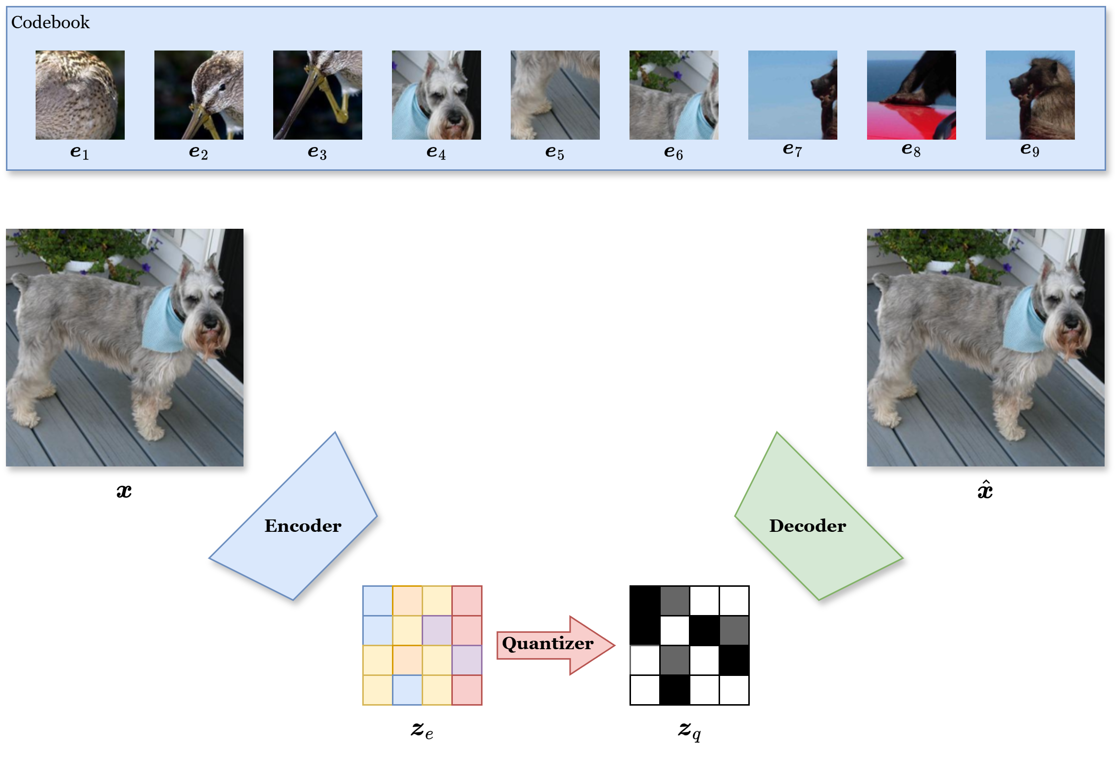
Fig. 22 The working mechanism of VQ-VAE.

The training objective has three parts. If \(D_\theta\) is the decoder, the reconstruction term is

\[ \mathcal{L}_{rec} = - \log p_\theta(\boldsymbol{x} | \boldsymbol{z}_q(\boldsymbol{x})). \]

The codebook loss moves the selected embedding vectors toward the encoder outputs:

\[ \mathcal{L}_{codebook} = \left\| \operatorname{sg}\left[\boldsymbol{z}_e(\boldsymbol{x})\right] - \boldsymbol{z}_q(\boldsymbol{x}) \right\|_2^2. \]

The stop-gradient operator \(\operatorname{sg}[\cdot]\) means that this term updates the codebook but not the encoder. The commitment loss moves the encoder outputs toward the selected embeddings:

\[ \mathcal{L}_{commit} = \left\| \boldsymbol{z}_e(\boldsymbol{x}) - \operatorname{sg}\left[\boldsymbol{z}_q(\boldsymbol{x})\right] \right\|_2^2. \]

The full loss used in the implementation is

\[ \mathcal{L}_{VQ} = \mathcal{L}_{rec} + \mathcal{L}_{codebook} + \beta_{commit}\mathcal{L}_{commit}. \]

The commitment term is not a cosmetic detail. Without it, the encoder can keep moving its outputs around the continuous space while the codebook chases them. The quantizer then becomes unstable, codes can be used inconsistently, and the decoder receives a moving symbolic language. The commitment term asks the encoder to commit to the vocabulary it is learning to use.

A complete VQ-VAE generative model has two stages. The first stage is an autoencoding stage: it learns the encoder, codebook, and decoder. This stage tells us how to convert an image into a grid of discrete indices and how to decode such a grid back into an image. However, this alone is not enough for unconditional generation. It only gives a tokenizer and a detokenizer. To generate new images, we still need to know which grids of indices are likely.

This distinction is crucial. If we sample each code independently from its marginal frequency, we preserve only how often each code appears. We destroy spatial dependence. A code that often appears near the boundary of a shoe may be sampled in the middle of the background. A code that represents a local texture may be placed next to incompatible neighboring codes. The decoder will still produce an image, but the image will usually be poor because the latent grid is not a plausible encoded Fashion MNIST image.

The second stage therefore learns a prior over code grids:

\[ p_\psi(\boldsymbol{k}) = \prod_{i,j} p_\psi(k_{i,j} | k_{<i,j}), \]

where \(\boldsymbol{k}\) is the grid of discrete indices and \(k_{<i,j}\) denotes the previously generated positions in raster order. In the code below this prior is a small PixelCNN. The masks in the convolutional layers enforce the autoregressive rule: when predicting the code at one location, the network can only use earlier locations. Sampling then proceeds one position at a time. The PixelCNN samples the code grid, and the VQ-VAE decoder maps the sampled codebook vectors into an image.

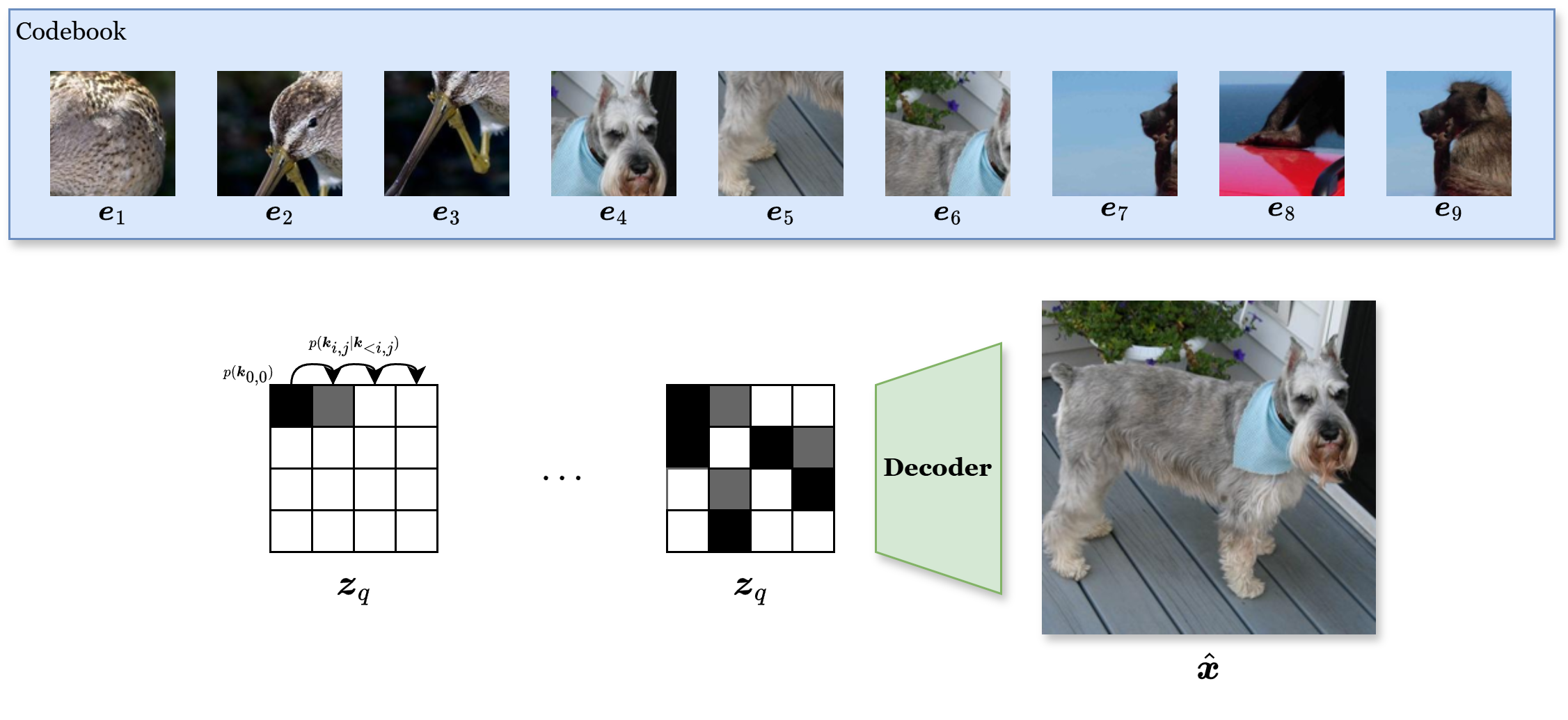
Fig. 23 Sampling VQ-VAE using PixelCNN.

This also clarifies why VQ-VAE can solve some vanilla VAE weaknesses but creates new failure modes. It reduces the pressure to match every approximate posterior to a simple Gaussian prior, because the representation is discrete and the prior can be learned after the tokenizer. It can avoid some smooth averaging because the decoder sees selected visual tokens rather than noisy Gaussian samples. But codebook collapse can still happen: if only a few codebook entries are used, the discrete vocabulary is mostly dead. Prior mismatch can also still happen: if the PixelCNN prior learns the code-grid distribution poorly, reconstructions may look good while unconditional samples look bad. The code therefore reports code usage and trains the prior on codes produced by the same trained VQ-VAE.

The implementation below follows this two-stage structure. First, the VQ-VAE learns a discrete latent vocabulary and a decoder. Second, the training set is encoded into grids of code indices. Third, a PixelCNN prior is trained over those grids. Sampling independent code indices from a histogram is intentionally avoided because it removes the spatial structure that the decoder expects.

VQ-VAE in one line

The encoder produces continuous vectors, the quantizer replaces them with nearest codebook entries, the decoder reconstructs from those discrete codes, and a separate prior learns which code grids are plausible.

class VectorQuantizer(nn.Module):
    def __init__(self, num_embeddings=128, embedding_dim=64, commitment_cost=0.1):
        super().__init__()
        self.num_embeddings = num_embeddings
        self.embedding_dim = embedding_dim
        self.commitment_cost = commitment_cost
        self.codebook = nn.Embedding(num_embeddings, embedding_dim)
        nn.init.normal_(self.codebook.weight, mean=0.0, std=0.5)

    def forward(self, z_e):
        flat = z_e.permute(0, 2, 3, 1).contiguous().view(-1, self.embedding_dim)
        distances = (
            flat.pow(2).sum(1, keepdim=True)
            - 2 * flat @ self.codebook.weight.t()
            + self.codebook.weight.pow(2).sum(1)
        )
        indices = distances.argmin(dim=1)
        z_q = self.codebook(indices).view(z_e.size(0), z_e.size(2), z_e.size(3), self.embedding_dim)
        z_q = z_q.permute(0, 3, 1, 2).contiguous()

        codebook_loss = F.mse_loss(z_e.detach(), z_q)
        commitment_loss = F.mse_loss(z_e, z_q.detach())
        loss = codebook_loss + self.commitment_cost * commitment_loss

        encodings = F.one_hot(indices, self.num_embeddings).float()
        avg_probs = encodings.mean(dim=0)
        perplexity = torch.exp(-torch.sum(avg_probs * torch.log(avg_probs + 1e-10)))

        z_q = z_e + (z_q - z_e).detach()
        return z_q, loss, indices.view(z_e.size(0), z_e.size(2), z_e.size(3)), perplexity


class VQResidualBlock(nn.Module):
    def __init__(self, channels):
        super().__init__()
        self.net = nn.Sequential(
            nn.Conv2d(channels, channels, kernel_size=3, padding=1),
            nn.ReLU(True),
            nn.Conv2d(channels, channels, kernel_size=1),
        )

    def forward(self, x):
        return F.relu(x + self.net(x), inplace=True)


class VQVAE(nn.Module):
    def __init__(self, embedding_dim=64, num_embeddings=128, base_channels=64):
        super().__init__()
        self.encoder = nn.Sequential(
            nn.Conv2d(1, base_channels, kernel_size=4, stride=2, padding=1),
            nn.ReLU(True),
            VQResidualBlock(base_channels),
            nn.Conv2d(base_channels, base_channels * 2, kernel_size=4, stride=2, padding=1),
            nn.ReLU(True),
            VQResidualBlock(base_channels * 2),
            nn.Conv2d(base_channels * 2, embedding_dim, kernel_size=1),
        )
        self.quantizer = VectorQuantizer(num_embeddings=num_embeddings, embedding_dim=embedding_dim)
        self.decoder = nn.Sequential(
            nn.Conv2d(embedding_dim, base_channels * 2, kernel_size=3, padding=1),
            nn.ReLU(True),
            VQResidualBlock(base_channels * 2),
            nn.ConvTranspose2d(base_channels * 2, base_channels, kernel_size=4, stride=2, padding=1),
            nn.ReLU(True),
            VQResidualBlock(base_channels),
            nn.ConvTranspose2d(base_channels, 1, kernel_size=4, stride=2, padding=1),
        )

    def forward(self, x):
        z_e = self.encoder(x)
        z_q, vq_loss, indices, perplexity = self.quantizer(z_e)
        logits = self.decoder(z_q)
        return logits, vq_loss, indices, perplexity


class MaskedConv2d(nn.Conv2d):
    def __init__(self, mask_type, *args, **kwargs):
        super().__init__(*args, **kwargs)
        self.register_buffer("mask", torch.ones_like(self.weight))
        _, _, h, w = self.weight.shape
        self.mask[:, :, h // 2, w // 2 + (mask_type == "B") :] = 0
        self.mask[:, :, h // 2 + 1 :] = 0

    def forward(self, x):
        return F.conv2d(
            x,
            self.weight * self.mask,
            self.bias,
            self.stride,
            self.padding,
            self.dilation,
            self.groups,
        )


class PixelCNNPrior(nn.Module):
    def __init__(self, num_embeddings, hidden_channels=192, num_layers=6):
        super().__init__()
        self.embedding = nn.Embedding(num_embeddings, hidden_channels)
        layers = [MaskedConv2d("A", hidden_channels, hidden_channels, kernel_size=5, padding=2), nn.ReLU(True)]
        for _ in range(num_layers - 1):
            layers += [MaskedConv2d("B", hidden_channels, hidden_channels, kernel_size=3, padding=1), nn.ReLU(True)]
        layers.append(nn.Conv2d(hidden_channels, num_embeddings, kernel_size=1))
        self.net = nn.Sequential(*layers)

    def forward(self, indices):
        x = self.embedding(indices).permute(0, 3, 1, 2).contiguous()
        return self.net(x)


@torch.no_grad()
def encode_dataset_to_indices(model, loader, device):
    model.eval()
    all_indices = []
    for x, _ in tqdm(loader, desc="encode codes", leave=False):
        x = x.to(device)
        _, _, indices, _ = model(x)
        all_indices.append(indices.cpu())
    return torch.cat(all_indices, dim=0)


vqvae = VQVAE(embedding_dim=64, num_embeddings=128, base_channels=64).to(device)
vq_optimizer = torch.optim.Adam(vqvae.parameters(), lr=2e-4)
vq_epochs = 80
for epoch in tqdm(range(vq_epochs), desc="VQ-VAE epochs"):
    vqvae.train()
    running = 0.0
    running_recon = 0.0
    running_vq = 0.0
    running_perplexity = 0.0
    for x, _ in tqdm(train_loader, desc="VQ train", leave=False):
        x = x.to(device)
        vq_optimizer.zero_grad()
        logits, vq_loss, _, perplexity = vqvae(x)
        recon = F.binary_cross_entropy_with_logits(logits, x, reduction="mean")
        loss = recon + vq_loss
        loss.backward()
        torch.nn.utils.clip_grad_norm_(vqvae.parameters(), max_norm=1.0)
        vq_optimizer.step()
        running += loss.item()
        running_recon += recon.item()
        running_vq += vq_loss.item()
        running_perplexity += perplexity.item()
    print(
        f"Epoch {epoch + 1:02d} | VQ-VAE loss: {running / len(train_loader):.4f} | "
        f"recon: {running_recon / len(train_loader):.4f} | "
        f"vq: {running_vq / len(train_loader):.4f} | "
        f"perplexity: {running_perplexity / len(train_loader):.1f}"
    )


train_code_indices = encode_dataset_to_indices(vqvae, train_loader, device)
test_code_indices = encode_dataset_to_indices(vqvae, test_loader, device)
code_height, code_width = train_code_indices.shape[1:]

prior_train_loader = DataLoader(
    TensorDataset(train_code_indices.long()),
    batch_size=256,
    shuffle=True,
    num_workers=0,
)
prior_test_loader = DataLoader(
    TensorDataset(test_code_indices.long()),
    batch_size=256,
    shuffle=False,
    num_workers=0,
)

pixel_prior = PixelCNNPrior(vqvae.quantizer.num_embeddings).to(device)
prior_optimizer = torch.optim.Adam(pixel_prior.parameters(), lr=2e-4)
prior_epochs = 60
for epoch in tqdm(range(prior_epochs), desc="PixelCNN prior epochs"):
    pixel_prior.train()
    running = 0.0
    for (indices,) in tqdm(prior_train_loader, desc="prior train", leave=False):
        indices = indices.to(device)
        prior_optimizer.zero_grad()
        logits = pixel_prior(indices)
        loss = F.cross_entropy(logits, indices)
        loss.backward()
        torch.nn.utils.clip_grad_norm_(pixel_prior.parameters(), max_norm=1.0)
        prior_optimizer.step()
        running += loss.item()
    prior_eval = 0.0
    pixel_prior.eval()
    for (indices,) in prior_test_loader:
        indices = indices.to(device)
        logits = pixel_prior(indices)
        prior_eval += F.cross_entropy(logits, indices).item()
    prior_eval /= len(prior_test_loader)
    print(f"Epoch {epoch + 1:02d} | prior nll: {running / len(prior_train_loader):.4f} | val nll: {prior_eval:.4f}")


@torch.no_grad()
def sample_vqvae_with_prior(model, prior, n=16, temperature=0.85, top_k=40, visualize=False):
    model.eval()
    prior.eval()
    indices = torch.zeros(n, code_height, code_width, dtype=torch.long, device=device)
    for row in range(code_height):
        for col in range(code_width):
            logits = prior(indices)[:, :, row, col] / temperature
            if top_k is not None:
                values, choices = logits.topk(k=min(top_k, logits.size(1)), dim=1)
                probs = torch.softmax(values, dim=1)
                selected = torch.multinomial(probs, num_samples=1)
                indices[:, row, col] = choices.gather(1, selected).squeeze(1)
            else:
                probs = torch.softmax(logits, dim=1)
                indices[:, row, col] = torch.multinomial(probs, num_samples=1).squeeze(1)
    z_q = model.quantizer.codebook(indices.view(-1)).view(
        n, code_height, code_width, model.quantizer.embedding_dim
    )
    z_q = z_q.permute(0, 3, 1, 2).contiguous()
    logits = model.decoder(z_q)
    samples = torch.sigmoid(logits)
    if visualize:
        image = utils.make_grid(samples.cpu(), nrow=4, pad_value=1.0)
        plt.figure(figsize=(6, 6))
        plt.imshow(image.permute(1, 2, 0), cmap="gray")
        plt.axis("off")
        plt.show()
    return samples

Epoch 01 | VQ-VAE loss: 1.1605 | recon: 0.3588 | vq: 0.8017 | perplexity: 2.8

Epoch 02 | VQ-VAE loss: 0.7199 | recon: 0.2955 | vq: 0.4244 | perplexity: 5.0

Epoch 03 | VQ-VAE loss: 0.6356 | recon: 0.2875 | vq: 0.3482 | perplexity: 5.6

Epoch 04 | VQ-VAE loss: 0.5935 | recon: 0.2830 | vq: 0.3105 | perplexity: 5.9

Epoch 05 | VQ-VAE loss: 0.5668 | recon: 0.2804 | vq: 0.2864 | perplexity: 6.2

Epoch 06 | VQ-VAE loss: 0.5408 | recon: 0.2779 | vq: 0.2629 | perplexity: 6.8

Epoch 07 | VQ-VAE loss: 0.4928 | recon: 0.2746 | vq: 0.2182 | perplexity: 8.1

Epoch 08 | VQ-VAE loss: 0.4519 | recon: 0.2724 | vq: 0.1795 | perplexity: 8.6

Epoch 09 | VQ-VAE loss: 0.4308 | recon: 0.2710 | vq: 0.1598 | perplexity: 8.9

Epoch 10 | VQ-VAE loss: 0.4162 | recon: 0.2700 | vq: 0.1462 | perplexity: 9.1

Epoch 11 | VQ-VAE loss: 0.4079 | recon: 0.2693 | vq: 0.1387 | perplexity: 9.2

Epoch 12 | VQ-VAE loss: 0.4027 | recon: 0.2687 | vq: 0.1340 | perplexity: 9.3

Epoch 13 | VQ-VAE loss: 0.3995 | recon: 0.2682 | vq: 0.1313 | perplexity: 9.4

Epoch 14 | VQ-VAE loss: 0.3961 | recon: 0.2676 | vq: 0.1284 | perplexity: 9.6

Epoch 15 | VQ-VAE loss: 0.3887 | recon: 0.2668 | vq: 0.1219 | perplexity: 10.2

Epoch 16 | VQ-VAE loss: 0.3786 | recon: 0.2660 | vq: 0.1126 | perplexity: 10.6

Epoch 17 | VQ-VAE loss: 0.3743 | recon: 0.2655 | vq: 0.1088 | perplexity: 10.7

Epoch 18 | VQ-VAE loss: 0.3721 | recon: 0.2652 | vq: 0.1069 | perplexity: 10.8

Epoch 19 | VQ-VAE loss: 0.3698 | recon: 0.2647 | vq: 0.1051 | perplexity: 11.2

Epoch 20 | VQ-VAE loss: 0.3660 | recon: 0.2643 | vq: 0.1017 | perplexity: 11.5

Epoch 21 | VQ-VAE loss: 0.3618 | recon: 0.2638 | vq: 0.0980 | perplexity: 11.8

Epoch 22 | VQ-VAE loss: 0.3585 | recon: 0.2635 | vq: 0.0950 | perplexity: 11.9

Epoch 23 | VQ-VAE loss: 0.3568 | recon: 0.2632 | vq: 0.0935 | perplexity: 12.1

Epoch 24 | VQ-VAE loss: 0.3557 | recon: 0.2629 | vq: 0.0928 | perplexity: 12.3

Epoch 25 | VQ-VAE loss: 0.3532 | recon: 0.2626 | vq: 0.0906 | perplexity: 12.8

Epoch 26 | VQ-VAE loss: 0.3492 | recon: 0.2621 | vq: 0.0870 | perplexity: 13.6

Epoch 27 | VQ-VAE loss: 0.3446 | recon: 0.2616 | vq: 0.0830 | perplexity: 14.1

Epoch 28 | VQ-VAE loss: 0.3421 | recon: 0.2614 | vq: 0.0807 | perplexity: 14.4

Epoch 29 | VQ-VAE loss: 0.3409 | recon: 0.2611 | vq: 0.0798 | perplexity: 14.5

Epoch 30 | VQ-VAE loss: 0.3407 | recon: 0.2609 | vq: 0.0799 | perplexity: 14.7

Epoch 31 | VQ-VAE loss: 0.3409 | recon: 0.2607 | vq: 0.0801 | perplexity: 14.8

Epoch 32 | VQ-VAE loss: 0.3403 | recon: 0.2605 | vq: 0.0798 | perplexity: 15.0

Epoch 33 | VQ-VAE loss: 0.3398 | recon: 0.2603 | vq: 0.0795 | perplexity: 15.1

Epoch 34 | VQ-VAE loss: 0.3397 | recon: 0.2601 | vq: 0.0795 | perplexity: 15.2

Epoch 35 | VQ-VAE loss: 0.3399 | recon: 0.2600 | vq: 0.0800 | perplexity: 15.3

Epoch 36 | VQ-VAE loss: 0.3403 | recon: 0.2599 | vq: 0.0804 | perplexity: 15.4

Epoch 37 | VQ-VAE loss: 0.3407 | recon: 0.2597 | vq: 0.0810 | perplexity: 15.6

Epoch 38 | VQ-VAE loss: 0.3410 | recon: 0.2595 | vq: 0.0814 | perplexity: 15.8

Epoch 39 | VQ-VAE loss: 0.3413 | recon: 0.2594 | vq: 0.0819 | perplexity: 16.1

Epoch 40 | VQ-VAE loss: 0.3406 | recon: 0.2592 | vq: 0.0814 | perplexity: 16.5

Epoch 41 | VQ-VAE loss: 0.3383 | recon: 0.2590 | vq: 0.0793 | perplexity: 16.9

Epoch 42 | VQ-VAE loss: 0.3360 | recon: 0.2588 | vq: 0.0772 | perplexity: 17.3

Epoch 43 | VQ-VAE loss: 0.3348 | recon: 0.2586 | vq: 0.0762 | perplexity: 17.5

Epoch 44 | VQ-VAE loss: 0.3349 | recon: 0.2585 | vq: 0.0764 | perplexity: 17.7

Epoch 45 | VQ-VAE loss: 0.3351 | recon: 0.2584 | vq: 0.0767 | perplexity: 17.8

Epoch 46 | VQ-VAE loss: 0.3355 | recon: 0.2583 | vq: 0.0771 | perplexity: 18.0

Epoch 47 | VQ-VAE loss: 0.3350 | recon: 0.2582 | vq: 0.0768 | perplexity: 18.3

Epoch 48 | VQ-VAE loss: 0.3337 | recon: 0.2581 | vq: 0.0756 | perplexity: 18.6

Epoch 49 | VQ-VAE loss: 0.3326 | recon: 0.2580 | vq: 0.0747 | perplexity: 18.8

Epoch 50 | VQ-VAE loss: 0.3323 | recon: 0.2579 | vq: 0.0744 | perplexity: 18.9

Epoch 51 | VQ-VAE loss: 0.3321 | recon: 0.2578 | vq: 0.0743 | perplexity: 19.1

Epoch 52 | VQ-VAE loss: 0.3316 | recon: 0.2577 | vq: 0.0739 | perplexity: 19.4

Epoch 53 | VQ-VAE loss: 0.3309 | recon: 0.2576 | vq: 0.0733 | perplexity: 19.6

Epoch 54 | VQ-VAE loss: 0.3302 | recon: 0.2575 | vq: 0.0727 | perplexity: 19.8

Epoch 55 | VQ-VAE loss: 0.3298 | recon: 0.2574 | vq: 0.0724 | perplexity: 20.0

Epoch 56 | VQ-VAE loss: 0.3291 | recon: 0.2573 | vq: 0.0718 | perplexity: 20.1

Epoch 57 | VQ-VAE loss: 0.3283 | recon: 0.2572 | vq: 0.0711 | perplexity: 20.3

Epoch 58 | VQ-VAE loss: 0.3279 | recon: 0.2571 | vq: 0.0708 | perplexity: 20.4

Epoch 59 | VQ-VAE loss: 0.3278 | recon: 0.2570 | vq: 0.0707 | perplexity: 20.5

Epoch 60 | VQ-VAE loss: 0.3277 | recon: 0.2570 | vq: 0.0707 | perplexity: 20.6

Epoch 61 | VQ-VAE loss: 0.3277 | recon: 0.2569 | vq: 0.0708 | perplexity: 20.7

Epoch 62 | VQ-VAE loss: 0.3275 | recon: 0.2569 | vq: 0.0707 | perplexity: 20.7

Epoch 63 | VQ-VAE loss: 0.3274 | recon: 0.2568 | vq: 0.0706 | perplexity: 20.8

Epoch 64 | VQ-VAE loss: 0.3273 | recon: 0.2568 | vq: 0.0705 | perplexity: 20.8

Epoch 65 | VQ-VAE loss: 0.3273 | recon: 0.2567 | vq: 0.0707 | perplexity: 20.8

Epoch 66 | VQ-VAE loss: 0.3271 | recon: 0.2566 | vq: 0.0705 | perplexity: 20.9

Epoch 67 | VQ-VAE loss: 0.3269 | recon: 0.2566 | vq: 0.0703 | perplexity: 21.0

Epoch 68 | VQ-VAE loss: 0.3268 | recon: 0.2565 | vq: 0.0703 | perplexity: 21.1

Epoch 69 | VQ-VAE loss: 0.3267 | recon: 0.2564 | vq: 0.0702 | perplexity: 21.3

Epoch 70 | VQ-VAE loss: 0.3264 | recon: 0.2564 | vq: 0.0700 | perplexity: 21.5

Epoch 71 | VQ-VAE loss: 0.3257 | recon: 0.2563 | vq: 0.0694 | perplexity: 21.6

Epoch 72 | VQ-VAE loss: 0.3255 | recon: 0.2563 | vq: 0.0692 | perplexity: 21.7

Epoch 73 | VQ-VAE loss: 0.3255 | recon: 0.2562 | vq: 0.0693 | perplexity: 21.7

Epoch 74 | VQ-VAE loss: 0.3256 | recon: 0.2562 | vq: 0.0694 | perplexity: 21.7

Epoch 75 | VQ-VAE loss: 0.3258 | recon: 0.2562 | vq: 0.0697 | perplexity: 21.7

Epoch 76 | VQ-VAE loss: 0.3259 | recon: 0.2561 | vq: 0.0698 | perplexity: 21.8

Epoch 77 | VQ-VAE loss: 0.3261 | recon: 0.2561 | vq: 0.0700 | perplexity: 21.8

Epoch 78 | VQ-VAE loss: 0.3263 | recon: 0.2560 | vq: 0.0702 | perplexity: 21.8

Epoch 79 | VQ-VAE loss: 0.3262 | recon: 0.2560 | vq: 0.0702 | perplexity: 21.8

Epoch 80 | VQ-VAE loss: 0.3263 | recon: 0.2560 | vq: 0.0703 | perplexity: 21.8

Epoch 01 | prior nll: 2.9723 | val nll: 2.4877

Epoch 02 | prior nll: 2.3082 | val nll: 2.1653

Epoch 03 | prior nll: 2.0968 | val nll: 2.0609

Epoch 04 | prior nll: 2.0115 | val nll: 2.0029

Epoch 05 | prior nll: 1.9562 | val nll: 1.9464

Epoch 06 | prior nll: 1.9133 | val nll: 1.9116

Epoch 07 | prior nll: 1.8824 | val nll: 1.8794

Epoch 08 | prior nll: 1.8578 | val nll: 1.8609

Epoch 09 | prior nll: 1.8350 | val nll: 1.8510

Epoch 10 | prior nll: 1.8160 | val nll: 1.8339

Epoch 11 | prior nll: 1.8004 | val nll: 1.8179

Epoch 12 | prior nll: 1.7857 | val nll: 1.8062

Epoch 13 | prior nll: 1.7731 | val nll: 1.7976

Epoch 14 | prior nll: 1.7614 | val nll: 1.7836

Epoch 15 | prior nll: 1.7512 | val nll: 1.7805

Epoch 16 | prior nll: 1.7421 | val nll: 1.7664

Epoch 17 | prior nll: 1.7338 | val nll: 1.7638

Epoch 18 | prior nll: 1.7253 | val nll: 1.7512

Epoch 19 | prior nll: 1.7179 | val nll: 1.7523

Epoch 20 | prior nll: 1.7113 | val nll: 1.7441

Epoch 21 | prior nll: 1.7051 | val nll: 1.7360

Epoch 22 | prior nll: 1.6996 | val nll: 1.7374

Epoch 23 | prior nll: 1.6930 | val nll: 1.7369

Epoch 24 | prior nll: 1.6883 | val nll: 1.7235

Epoch 25 | prior nll: 1.6830 | val nll: 1.7198

Epoch 26 | prior nll: 1.6775 | val nll: 1.7180

Epoch 27 | prior nll: 1.6731 | val nll: 1.7158

Epoch 28 | prior nll: 1.6692 | val nll: 1.7144

Epoch 29 | prior nll: 1.6652 | val nll: 1.7065

Epoch 30 | prior nll: 1.6612 | val nll: 1.7045

Epoch 31 | prior nll: 1.6567 | val nll: 1.7004

Epoch 32 | prior nll: 1.6536 | val nll: 1.6981

Epoch 33 | prior nll: 1.6497 | val nll: 1.6985

Epoch 34 | prior nll: 1.6454 | val nll: 1.6948

Epoch 35 | prior nll: 1.6424 | val nll: 1.6933

Epoch 36 | prior nll: 1.6391 | val nll: 1.6914

Epoch 37 | prior nll: 1.6361 | val nll: 1.6894

Epoch 38 | prior nll: 1.6331 | val nll: 1.6837

Epoch 39 | prior nll: 1.6300 | val nll: 1.6859

Epoch 40 | prior nll: 1.6263 | val nll: 1.6873

Epoch 41 | prior nll: 1.6246 | val nll: 1.6794

Epoch 42 | prior nll: 1.6214 | val nll: 1.6786

Epoch 43 | prior nll: 1.6182 | val nll: 1.6789

Epoch 44 | prior nll: 1.6159 | val nll: 1.6784

Epoch 45 | prior nll: 1.6133 | val nll: 1.6743

Epoch 46 | prior nll: 1.6110 | val nll: 1.6751

Epoch 47 | prior nll: 1.6086 | val nll: 1.6745

Epoch 48 | prior nll: 1.6063 | val nll: 1.6715

Epoch 49 | prior nll: 1.6036 | val nll: 1.6720

Epoch 50 | prior nll: 1.6015 | val nll: 1.6697

Epoch 51 | prior nll: 1.5994 | val nll: 1.6662

Epoch 52 | prior nll: 1.5974 | val nll: 1.6701

Epoch 53 | prior nll: 1.5948 | val nll: 1.6656

Epoch 54 | prior nll: 1.5927 | val nll: 1.6648

Epoch 55 | prior nll: 1.5905 | val nll: 1.6618

Epoch 56 | prior nll: 1.5893 | val nll: 1.6620

Epoch 57 | prior nll: 1.5864 | val nll: 1.6594

Epoch 58 | prior nll: 1.5850 | val nll: 1.6586

Epoch 59 | prior nll: 1.5828 | val nll: 1.6600

Epoch 60 | prior nll: 1.5812 | val nll: 1.6584

@torch.no_grad()
def collect_code_statistics(model, loader, device):
    counts = torch.zeros(model.quantizer.num_embeddings, device=device)
    model.eval()
    for x, _ in tqdm(loader, desc="code usage", leave=False):
        x = x.to(device)
        _, _, indices, _ = model(x)
        counts += torch.bincount(indices.reshape(-1), minlength=model.quantizer.num_embeddings).float()
    probs = counts / counts.sum()
    active_codes = int((counts > 0).sum().item())
    usage_perplexity = torch.exp(-torch.sum(probs * torch.log(probs + 1e-10))).item()
    return {"active_codes": active_codes, "usage_perplexity": usage_perplexity}


vq_code_stats = collect_code_statistics(vqvae, train_loader, device)
print(vq_code_stats)

{'active_codes': 37, 'usage_perplexity': 21.857250213623047}

Once the prior is trained, VQ-VAE becomes a real two-stage generative pipeline rather than just an autoencoding tokenizer. The first stage learns the map

\[ \boldsymbol{x} \longmapsto \boldsymbol{k}(\boldsymbol{x}) \longmapsto \hat{\boldsymbol{x}}, \]

where \(\boldsymbol{k}(\boldsymbol{x})\) is a grid of discrete code indices. The second stage learns how to sample plausible \(\boldsymbol{k}\) grids without seeing the original image. This separation exposes two different questions that are entangled in a vanilla VAE. The first question is representation learning: can the model describe an image with a compact latent object? The second question is generative modeling: can the model sample latent objects that look like the ones produced by real images?

The code-usage diagnostic is included for the same reason that KL diagnostics are included for Gaussian VAEs. In a Gaussian VAE, a latent coordinate can become inactive when its approximate posterior remains close to the prior for every input. In VQ-VAE, a codebook vector can become inactive when no encoder output selects it. Both cases are forms of unused latent capacity. They are not mathematically identical, but they express the same practical warning: the architecture may contain a large latent space while the trained model uses only a small part of it.

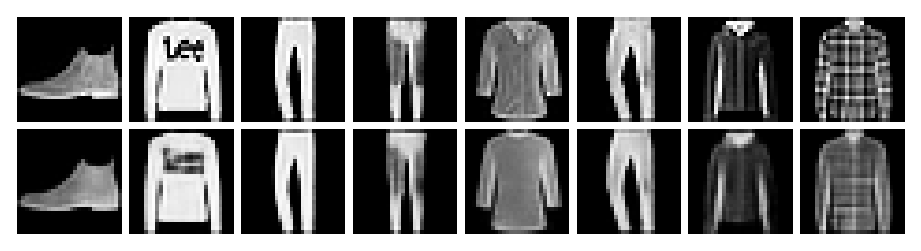
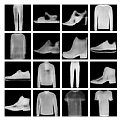
The prior diagnostic is equally important. Good reconstructions do not imply good samples. Reconstructions use code grids obtained from real images, while generation uses code grids sampled from the learned prior. If the PixelCNN prior is weak, the sampled grids will not resemble encoded training grids, and the decoder will turn implausible latent syntax into implausible images. The implementation therefore uses a single trained VQ-VAE, measures code usage, trains the PixelCNN on that same model’s codes, and samples with a mildly tempered top-k distribution to avoid very unlikely code choices.

@torch.no_grad()
def show_vqvae_reconstructions(model, loader, device, n=8):
    model.eval()
    x, _ = next(iter(loader))
    x = x[:n].to(device)
    logits, _, _, _ = model(x)
    recon = torch.sigmoid(logits).cpu()
    grid = utils.make_grid(torch.cat([x.cpu(), recon], dim=0), nrow=n, pad_value=1.0)
    plt.figure(figsize=(1.5 * n, 3.0))
    plt.imshow(grid.permute(1, 2, 0), cmap="gray")
    plt.axis("off")
    plt.show()


show_vqvae_reconstructions(vqvae, test_loader, device)
sample_vqvae_with_prior(vqvae, pixel_prior, n=16, visualize=True)

tensor([[[[1.8388e-06, 8.7527e-07, 1.6401e-06,  ..., 4.9438e-08,
           5.1605e-07, 2.6850e-07],
          [1.9706e-07, 2.4110e-07, 1.3144e-06,  ..., 1.4650e-08,
           2.2133e-07, 8.7189e-08],
          [4.5099e-07, 3.7487e-07, 1.0401e-06,  ..., 5.9686e-09,
           1.1103e-06, 4.4317e-08],
          ...,
          [2.2583e-06, 4.8267e-07, 4.0752e-06,  ..., 2.3749e-08,
           2.5511e-07, 1.7993e-08],
          [3.1515e-07, 9.4032e-08, 3.2839e-07,  ..., 1.8399e-07,
           5.6140e-07, 7.0167e-08],
          [1.9027e-06, 4.5928e-07, 1.6511e-06,  ..., 5.1731e-07,
           2.2195e-06, 2.3041e-06]]],


        [[[3.1636e-07, 1.0489e-08, 2.9412e-08,  ..., 5.9324e-09,
           8.1758e-08, 2.4147e-07],
          [7.9983e-07, 9.3212e-08, 5.4065e-08,  ..., 2.5230e-08,
           7.3933e-07, 4.6091e-07],
          [8.6812e-08, 2.2255e-08, 1.9605e-06,  ..., 4.1074e-08,
           1.9353e-06, 9.7186e-07],
          ...,
          [3.9454e-05, 1.0206e-05, 5.5081e-07,  ..., 2.7740e-08,
           5.4849e-08, 1.3117e-07],
          [6.3848e-06, 3.3976e-06, 3.4888e-06,  ..., 1.4326e-07,
           1.5913e-07, 4.4649e-07],
          [8.6075e-06, 1.2228e-06, 1.9759e-06,  ..., 6.2197e-08,
           8.1312e-07, 4.0979e-06]]],


        [[[2.2423e-07, 3.8571e-09, 1.6388e-08,  ..., 5.4399e-08,
           7.9070e-07, 1.9466e-06],
          [2.2010e-07, 2.5025e-08, 2.1586e-08,  ..., 9.1665e-07,
           3.4468e-06, 4.8865e-06],
          [1.3076e-08, 5.9521e-09, 3.3597e-07,  ..., 7.7986e-06,
           1.2925e-05, 9.3096e-06],
          ...,
          [5.3677e-05, 1.6532e-05, 6.7088e-05,  ..., 4.1043e-05,
           3.1462e-05, 5.0771e-06],
          [1.4889e-05, 1.5112e-05, 3.8380e-05,  ..., 1.0271e-05,
           1.0728e-04, 2.2100e-05],
          [2.3690e-05, 1.3504e-05, 2.0557e-06,  ..., 2.1984e-05,
           5.7610e-05, 2.3126e-05]]],


        ...,


        [[[1.0094e-05, 1.3279e-06, 5.3489e-05,  ..., 6.6519e-05,
           9.5971e-06, 2.1973e-05],
          [6.8877e-06, 1.2994e-06, 2.6983e-05,  ..., 8.8679e-05,
           1.8907e-05, 2.6916e-05],
          [1.0923e-05, 1.5075e-06, 2.9866e-05,  ..., 3.4233e-04,
           1.2825e-04, 1.4862e-04],
          ...,
          [4.0620e-06, 1.0505e-06, 2.3703e-06,  ..., 3.8578e-01,
           1.5110e-03, 8.0189e-05],
          [4.2654e-06, 4.9652e-06, 1.0194e-05,  ..., 4.6986e-01,
           3.6812e-03, 1.7995e-04],
          [2.7483e-06, 1.2979e-06, 3.7116e-06,  ..., 2.5268e-01,
           2.0956e-03, 3.1973e-04]]],


        [[[3.8322e-05, 1.2447e-05, 2.4100e-04,  ..., 4.9385e-06,
           3.7983e-06, 1.8420e-06],
          [3.0391e-05, 1.0231e-05, 1.0356e-04,  ..., 4.1097e-05,
           2.7563e-05, 1.9108e-05],
          [5.6110e-05, 1.1481e-05, 1.2183e-04,  ..., 1.3130e-04,
           5.4124e-05, 2.9557e-05],
          ...,
          [6.1117e-06, 2.9980e-06, 3.5715e-05,  ..., 1.0566e-05,
           1.2735e-04, 3.6803e-06],
          [1.4826e-06, 4.5923e-07, 1.2536e-05,  ..., 3.8498e-06,
           6.0204e-05, 5.1206e-06],
          [2.7898e-06, 6.7195e-07, 1.9151e-05,  ..., 1.2166e-05,
           1.1519e-04, 2.7329e-05]]],


        [[[2.2322e-05, 1.1814e-06, 2.5360e-04,  ..., 2.5350e-06,
           2.4663e-06, 2.4640e-06],
          [8.5453e-06, 5.2936e-07, 1.0372e-05,  ..., 6.1343e-05,
           4.1268e-06, 1.4002e-06],
          [1.7313e-05, 1.9936e-06, 5.4660e-05,  ..., 1.8576e-04,
           7.6985e-06, 2.9251e-07],
          ...,
          [1.3007e-06, 5.0206e-07, 6.4620e-06,  ..., 3.2008e-07,
           5.4452e-06, 4.4618e-08],
          [1.2713e-07, 3.6649e-08, 9.2454e-07,  ..., 8.2385e-07,
           1.5204e-06, 4.8349e-08],
          [1.7071e-06, 3.2403e-07, 1.5398e-06,  ..., 2.3775e-06,
           4.8401e-06, 2.2146e-06]]]], device='cuda:0')

Conditional VAEs and the Move to Controlled Generation

The variants considered so far still model the unconditional data distribution \(p_{gt}(\boldsymbol{x})\). A conditional VAE changes the question. Instead of asking the model to generate a plausible image with no further instruction, we ask it to generate a plausible image given side information \(\boldsymbol{y}\). For Fashion MNIST, \(\boldsymbol{y}\) is the class label. The model should generate an ankle boot when \(\boldsymbol{y}\) says ankle boot, a shirt when \(\boldsymbol{y}\) says shirt, and so on. The remaining latent variable should represent variability inside the chosen class: style, thickness, pose, local shape, and other factors not specified by the label.

The conditional generative model is

\[ p_\theta(\boldsymbol{x},\boldsymbol{z}|\boldsymbol{y}) = p(\boldsymbol{z}|\boldsymbol{y}) p_\theta(\boldsymbol{x}|\boldsymbol{z},\boldsymbol{y}). \]

In the simplest implementation, the prior is still \(p(\boldsymbol{z}|\boldsymbol{y}) = \mathcal{N}(\boldsymbol{0},\boldsymbol{I})\), so the label changes only the encoder and decoder inputs. More expressive conditional VAEs can also learn a label-dependent prior. The approximate posterior becomes

\[ q_\phi(\boldsymbol{z}|\boldsymbol{x},\boldsymbol{y}), \]

and the conditional ELBO is

\[ \log p_\theta(\boldsymbol{x}|\boldsymbol{y}) \geq \mathbb{E}_{q_\phi(\boldsymbol{z}|\boldsymbol{x},\boldsymbol{y})} \left[ \log p_\theta(\boldsymbol{x}|\boldsymbol{z},\boldsymbol{y}) \right] - D_{KL}\left( q_\phi(\boldsymbol{z}|\boldsymbol{x},\boldsymbol{y}) \| p(\boldsymbol{z}|\boldsymbol{y}) \right). \]

This is the same variational argument as before, but applied to a conditional likelihood. The label is not an afterthought added to the generated image. It is part of the probabilistic model. The decoder is explicitly trained to explain \(\boldsymbol{x}\) using both \(\boldsymbol{z}\) and \(\boldsymbol{y}\), while the encoder learns the posterior over residual factors that remain uncertain after observing the label.

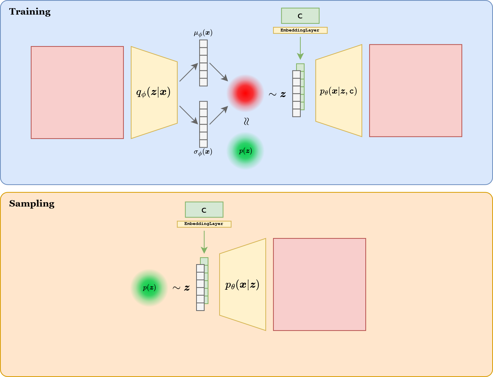
Fig. 24 The mechanism of Conditional VAE.

From the motivational perspective, a conditional VAE separates what should be controlled from what should remain random. In an unconditional VAE, class identity and within-class style compete for the same latent capacity. Some latent coordinates may encode whether the image is a sandal or a coat, while others encode details inside the class. In a conditional VAE, the class is provided directly. This frees the latent variable to focus on intra-class variation. This is why conditional generation is often visually cleaner than unconditional generation with the same network size.

This also addresses a different limitation of vanilla VAEs. The vanilla model may generate a plausible image, but it gives the user little control over what kind of image appears. Conditional VAEs, introduced in the broader conditional deep generative modeling literature [SLY15], turn generation into an input-output problem: choose a condition, sample a latent vector, decode. The cost is that the model now depends on the availability and quality of the conditioning variable. If the labels are noisy, incomplete, or too coarse, the conditional model inherits those limitations.

num_classes = 10


class ConditionalVAE(nn.Module):
    def __init__(self, latent_dim=32, base_channels=32, num_classes=10, label_dim=16):
        super().__init__()
        self.label_embed = nn.Embedding(num_classes, label_dim)
        self.encoder = nn.Sequential(
            nn.Conv2d(1, base_channels, kernel_size=4, stride=2, padding=1),
            nn.SiLU(),
            nn.Conv2d(base_channels, base_channels * 2, kernel_size=4, stride=2, padding=1),
            nn.SiLU(),
            nn.Flatten(),
        )
        encoded_dim = base_channels * 2 * 7 * 7
        self.mu_head = nn.Linear(encoded_dim + label_dim, latent_dim)
        self.logvar_head = nn.Linear(encoded_dim + label_dim, latent_dim)
        self.decoder_input = nn.Linear(latent_dim + label_dim, base_channels * 4 * 7 * 7)
        self.decoder = nn.Sequential(
            nn.Unflatten(1, (base_channels * 4, 7, 7)),
            nn.ConvTranspose2d(base_channels * 4, base_channels * 2, kernel_size=4, stride=2, padding=1),
            nn.SiLU(),
            nn.ConvTranspose2d(base_channels * 2, base_channels, kernel_size=4, stride=2, padding=1),
            nn.SiLU(),
            nn.Conv2d(base_channels, 1, kernel_size=3, padding=1),
        )

    def encode(self, x, y):
        h = self.encoder(x)
        y_embed = self.label_embed(y)
        h = torch.cat([h, y_embed], dim=1)
        return self.mu_head(h), self.logvar_head(h)

    def reparameterize(self, mu, logvar):
        std = torch.exp(0.5 * logvar)
        return mu + std * torch.randn_like(std)

    def decode(self, z, y):
        y_embed = self.label_embed(y)
        h = self.decoder_input(torch.cat([z, y_embed], dim=1))
        return self.decoder(h)

    def forward(self, x, y):
        mu, logvar = self.encode(x, y)
        z = self.reparameterize(mu, logvar)
        logits = self.decode(z, y)
        return logits, mu, logvar


@torch.no_grad()
def sample_cvae(model, class_id, n, device):
    model.eval()
    labels = torch.full((n,), class_id, device=device, dtype=torch.long)
    z = torch.randn(n, latent_dim, device=device)
    logits = model.decode(z, labels)
    return torch.sigmoid(logits)


@torch.no_grad()
def sample_cvae_from_labels(model, labels, device):
    model.eval()
    z = torch.randn(labels.size(0), latent_dim, device=device)
    logits = model.decode(z, labels)
    return torch.sigmoid(logits)

def train_conditional_vae_epoch(model, loader, optimizer, device, beta=1.0, free_bits=0.0):
    model.train()
    total_loss = 0.0
    total_kl = 0.0

    for x, y in tqdm(loader, desc="cVAE train", leave=False):
        x = x.to(device)
        y = y.to(device)

        optimizer.zero_grad()
        logits, mu, logvar = model(x, y)
        loss, _, kl = beta_vae_loss(x, logits, mu, logvar, beta=beta, free_bits=free_bits)
        loss.backward()
        optimizer.step()

        total_loss += loss.item()
        total_kl += kl.item()

    n = len(loader.dataset)
    return {"loss": total_loss / n, "kl": total_kl / n}


@torch.no_grad()
def evaluate_conditional_vae(model, loader, device, beta=1.0, free_bits=0.0):
    model.eval()
    total_loss = 0.0
    total_kl = 0.0

    for x, y in loader:
        x = x.to(device)
        y = y.to(device)
        logits, mu, logvar = model(x, y)
        loss, _, kl = beta_vae_loss(x, logits, mu, logvar, beta=beta, free_bits=free_bits)
        total_loss += loss.item()
        total_kl += kl.item()

    n = len(loader.dataset)
    return {"loss": total_loss / n, "kl": total_kl / n}


conditional_epochs = 50
cvae = ConditionalVAE(
    latent_dim=latent_dim,
    base_channels=base_channels,
    num_classes=num_classes,
).to(device)
cvae_optimizer = torch.optim.Adam(cvae.parameters(), lr=lr)
conditional_history = {"train_loss": [], "val_loss": [], "beta": []}

for epoch in tqdm(range(conditional_epochs), desc="cVAE epochs"):
    beta_t = linear_beta_schedule(epoch, conditional_epochs, start=0.0, stop=1.0, warmup_fraction=0.4)
    train_stats = train_conditional_vae_epoch(cvae, train_loader, cvae_optimizer, device, beta=beta_t, free_bits=0.1)
    val_stats = evaluate_conditional_vae(cvae, test_loader, device, beta=beta_t, free_bits=0.1)

    conditional_history["train_loss"].append(train_stats["loss"])
    conditional_history["val_loss"].append(val_stats["loss"])
    conditional_history["beta"].append(beta_t)

    print(
        f"Epoch {epoch + 1:02d} | beta: {beta_t:.2f} | "
        f"train loss: {train_stats['loss']:.4f} | val loss: {val_stats['loss']:.4f}"
    )

Epoch 01 | beta: 0.00 | train loss: 289.9086 | val loss: 239.6424

Epoch 02 | beta: 0.05 | train loss: 237.8366 | val loss: 233.5603

Epoch 03 | beta: 0.10 | train loss: 231.8255 | val loss: 230.6156

Epoch 04 | beta: 0.15 | train loss: 229.8014 | val loss: 230.0493

Epoch 05 | beta: 0.20 | train loss: 229.3547 | val loss: 229.9098

Epoch 06 | beta: 0.25 | train loss: 229.5029 | val loss: 230.3100

Epoch 07 | beta: 0.30 | train loss: 229.9132 | val loss: 230.8568

Epoch 08 | beta: 0.35 | train loss: 230.4245 | val loss: 231.4968

Epoch 09 | beta: 0.40 | train loss: 231.0201 | val loss: 232.2737

Epoch 10 | beta: 0.45 | train loss: 231.6346 | val loss: 232.8348

Epoch 11 | beta: 0.50 | train loss: 232.2457 | val loss: 233.6781

Epoch 12 | beta: 0.55 | train loss: 232.8843 | val loss: 234.4223

Epoch 13 | beta: 0.60 | train loss: 233.5197 | val loss: 235.0171

Epoch 14 | beta: 0.65 | train loss: 234.1204 | val loss: 235.6958

Epoch 15 | beta: 0.70 | train loss: 234.6985 | val loss: 236.3892

Epoch 16 | beta: 0.75 | train loss: 235.2812 | val loss: 236.9871

Epoch 17 | beta: 0.80 | train loss: 235.8874 | val loss: 237.6345

Epoch 18 | beta: 0.85 | train loss: 236.4044 | val loss: 238.2384

Epoch 19 | beta: 0.90 | train loss: 236.9444 | val loss: 238.6206

Epoch 20 | beta: 0.95 | train loss: 237.4700 | val loss: 239.1446

Epoch 21 | beta: 1.00 | train loss: 237.9145 | val loss: 239.5104

Epoch 22 | beta: 1.00 | train loss: 237.6416 | val loss: 239.4796

Epoch 23 | beta: 1.00 | train loss: 237.3964 | val loss: 239.1532

Epoch 24 | beta: 1.00 | train loss: 237.1215 | val loss: 238.8646

Epoch 25 | beta: 1.00 | train loss: 236.9002 | val loss: 238.7459

Epoch 26 | beta: 1.00 | train loss: 236.7143 | val loss: 238.5958

Epoch 27 | beta: 1.00 | train loss: 236.5232 | val loss: 238.3606

Epoch 28 | beta: 1.00 | train loss: 236.3845 | val loss: 238.2305

Epoch 29 | beta: 1.00 | train loss: 236.1943 | val loss: 238.1237

Epoch 30 | beta: 1.00 | train loss: 236.0484 | val loss: 237.8945

Epoch 31 | beta: 1.00 | train loss: 235.9238 | val loss: 237.7780

Epoch 32 | beta: 1.00 | train loss: 235.7247 | val loss: 237.5912

Epoch 33 | beta: 1.00 | train loss: 235.5968 | val loss: 237.5014

Epoch 34 | beta: 1.00 | train loss: 235.4866 | val loss: 237.4356

Epoch 35 | beta: 1.00 | train loss: 235.3591 | val loss: 237.3062

Epoch 36 | beta: 1.00 | train loss: 235.2524 | val loss: 237.1480

Epoch 37 | beta: 1.00 | train loss: 235.1470 | val loss: 237.0356

Epoch 38 | beta: 1.00 | train loss: 235.0175 | val loss: 236.9705

Epoch 39 | beta: 1.00 | train loss: 234.9341 | val loss: 236.8453

Epoch 40 | beta: 1.00 | train loss: 234.8093 | val loss: 236.8183

Epoch 41 | beta: 1.00 | train loss: 234.7831 | val loss: 236.6745

Epoch 42 | beta: 1.00 | train loss: 234.6452 | val loss: 236.5616

Epoch 43 | beta: 1.00 | train loss: 234.5467 | val loss: 236.5609

Epoch 44 | beta: 1.00 | train loss: 234.4556 | val loss: 236.5243

Epoch 45 | beta: 1.00 | train loss: 234.4064 | val loss: 236.5219

Epoch 46 | beta: 1.00 | train loss: 234.3241 | val loss: 236.2723

Epoch 47 | beta: 1.00 | train loss: 234.2571 | val loss: 236.3750

Epoch 48 | beta: 1.00 | train loss: 234.1784 | val loss: 236.1391

Epoch 49 | beta: 1.00 | train loss: 234.1319 | val loss: 236.1154

Epoch 50 | beta: 1.00 | train loss: 234.0209 | val loss: 236.0109

At this point, the label is not a decorative extra input. It changes the generative question from “draw any fashion item” to “draw a fashion item of the requested class.” The latent variable still matters, but its role changes: it no longer explains which class the object belongs to, because that part is already specified by the condition. Instead, it models the residual uncertainty inside the class.

This is why conditioning is so important conceptually. Once a condition is given, generation becomes a controlled mapping from a coarse semantic request plus latent noise to a concrete sample. In tiny form, that is already the same idea that later appears in text-guided image generation: the condition determines the semantic target, while the latent randomness governs the particular realization.

@torch.no_grad()
def show_cvae_class_samples(model, class_names, device, n_per_class=6):
    model.eval()
    rows = []
    for class_id, _ in enumerate(class_names):
        labels = torch.full((n_per_class,), class_id, device=device, dtype=torch.long)
        z = torch.randn(n_per_class, latent_dim, device=device)
        logits = model.decode(z, labels)
        rows.append(torch.sigmoid(logits).cpu())

    image = utils.make_grid(torch.cat(rows, dim=0), nrow=n_per_class, pad_value=1.0)
    plt.figure(figsize=(1.6 * n_per_class, 1.6 * len(class_names)))
    plt.imshow(image.permute(1, 2, 0), cmap="gray")
    plt.axis("off")
    plt.show()

    for class_id, name in enumerate(class_names):
        print(f"row {class_id}: {name}")


@torch.no_grad()
def interpolate_cvae_with_fixed_class(model, class_id, class_name, device, steps=8):
    model.eval()
    labels = torch.full((2,), class_id, device=device, dtype=torch.long)
    z0 = torch.randn(1, latent_dim, device=device)
    z1 = torch.randn(1, latent_dim, device=device)
    alphas = torch.linspace(0, 1, steps, device=device).view(-1, 1)
    z = (1 - alphas) * z0 + alphas * z1
    labels = torch.full((steps,), class_id, device=device, dtype=torch.long)
    logits = model.decode(z, labels)
    samples = torch.sigmoid(logits).cpu()
    image = utils.make_grid(samples, nrow=steps, pad_value=1.0)
    plt.figure(figsize=(1.7 * steps, 2.5))
    plt.imshow(image.permute(1, 2, 0), cmap="gray")
    plt.axis("off")
    plt.show()
    print(f"class-conditioned interpolation: {class_name}")


show_cvae_class_samples(cvae, train_dataset.classes, device, n_per_class=6)
interpolate_cvae_with_fixed_class(cvae, class_id=9, class_name=train_dataset.classes[9], device=device)

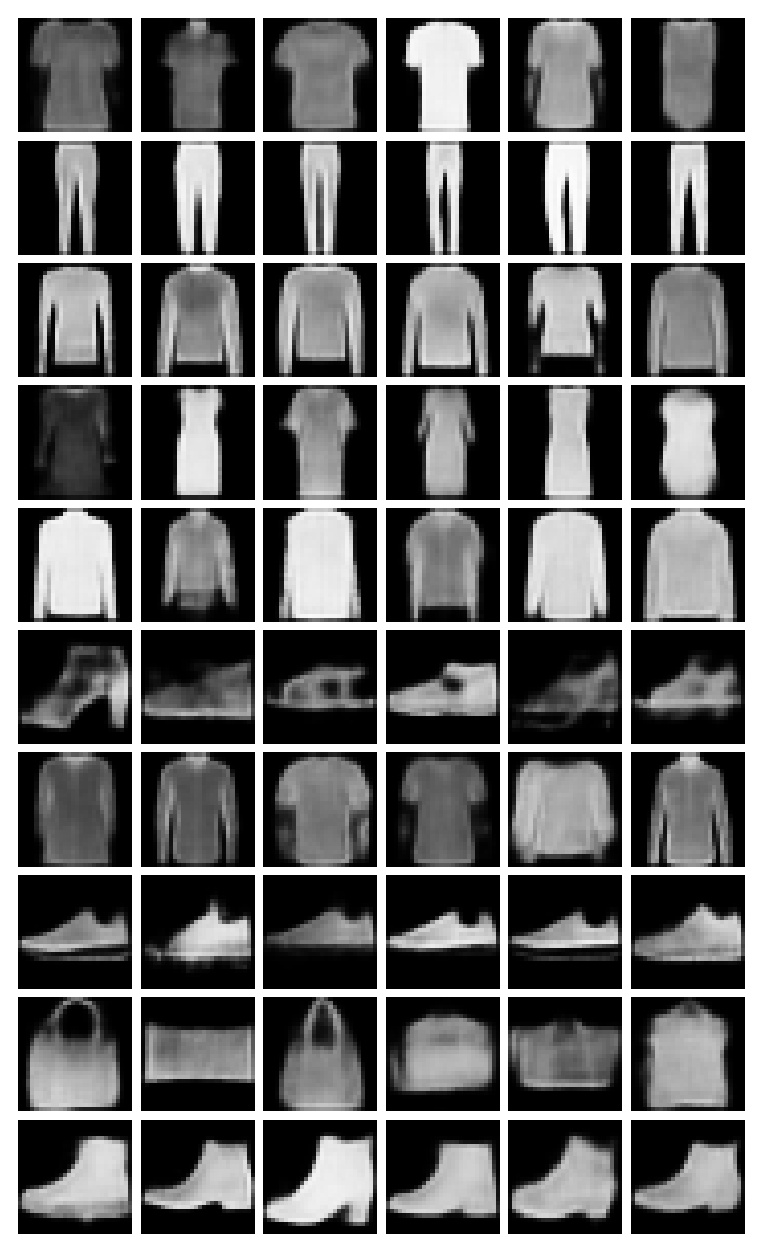
row 0: T-shirt/top
row 1: Trouser
row 2: Pullover
row 3: Dress
row 4: Coat
row 5: Sandal
row 6: Shirt
row 7: Sneaker
row 8: Bag
row 9: Ankle boot

class-conditioned interpolation: Ankle boot

The expected qualitative result is now stronger than in the unconditional case. Each row should stay semantically tied to its class, while still showing variability across columns. For instance, the Sandal row should not collapse to a single repeated template, and it should not drift into Sneaker or Ankle boot. If that happens, the model is either undertrained or not using the conditioning signal effectively.

The interpolation experiment adds a second check. By fixing the class and moving only in latent space, we can ask whether the model learned a smooth within-class manifold. A good result should morph one boot into another boot, not silently wander into a different class. That is exactly the decomposition we want: the label controls the semantic family, and the latent variable controls the instance-level variation inside that family.

Conditional generation

The condition specifies what should be controlled. The latent variable models what should remain variable inside that condition.

This methodological separation between condition information and residual uncertainty is the main reason conditional generative models became central in image generation. The condition specifies the part of the image distribution that should be controlled. The latent variable models the part that should remain diverse. In the Fashion MNIST example the condition is only a class label, but the same principle later appears with text prompts, segmentation maps, low-resolution images, edge maps, and other forms of guidance.

The conditional VAE also gives a useful warning. Adding labels does not automatically solve every VAE limitation. A weak decoder can still produce blurry samples. A badly weighted KL term can still underuse the latent variable. A condition that is too informative can even make the latent variable less necessary, because the decoder may explain most variation from \(\boldsymbol{y}\) alone. Therefore, the correct diagnostic question is not only whether the generated class is right. It is also whether samples within each class remain diverse and whether the latent variable actually controls meaningful residual variation.

Shared FID/KID Evaluation With Cached Real Features

All qualitative experiments above can be run variant by variant. For FID and KID, however, it is more efficient to centralize the evaluation and cache the real-data features once. This keeps the comparison focused on the generators rather than on repeated metric bookkeeping.

The progress bars below are written with explicit totals. This avoids the confusing behavior where a real-feature pass appears to stop at about one fifth of the dataloader simply because the function intentionally uses only the first num_real images and exits early.

from torchmetrics.image.fid import FrechetInceptionDistance
from torchmetrics.image.kid import KernelInceptionDistance


def prepare_for_inception_metrics(images):
    if images.size(1) == 1:
        images = images.repeat(1, 3, 1, 1)
    return images.clamp(0.0, 1.0)


@torch.no_grad()
def build_cached_real_metrics(real_loader, device, num_real=1000, metric_batch_size=64):
    fid = FrechetInceptionDistance(feature=2048, normalize=True, reset_real_features=False).set_dtype(torch.float64).to(device)
    kid = KernelInceptionDistance(feature=2048, subsets=10, subset_size=100, normalize=True, reset_real_features=False).to(device)
    seen = 0
    pbar = tqdm(total=num_real, desc="real metric cache")
    for real_images, _ in real_loader:
        remaining = num_real - seen
        if remaining <= 0:
            break
        batch_n = min(metric_batch_size, remaining, real_images.size(0))
        real_images = real_images[:batch_n].to(device)
        real_images = prepare_for_inception_metrics(real_images)
        fid.update(real_images, real=True)
        kid.update(real_images, real=True)
        seen += batch_n
        pbar.update(batch_n)
    pbar.close()
    return fid, kid


@torch.no_grad()
def evaluate_with_cached_real(sample_fn, base_fid, base_kid, num_fake=1000, metric_batch_size=64):
    fid = copy.deepcopy(base_fid)
    kid = copy.deepcopy(base_kid)
    generated = 0
    pbar = tqdm(total=num_fake, desc="fake metric pass")
    while generated < num_fake:
        batch_n = min(metric_batch_size, num_fake - generated)
        fake_images = prepare_for_inception_metrics(sample_fn(batch_n).to(device))
        fid.update(fake_images, real=False)
        kid.update(fake_images, real=False)
        generated += batch_n
        pbar.update(batch_n)
    pbar.close()
    kid_mean, kid_std = kid.compute()
    return {"fid": fid.compute().item(), "kid_mean": kid_mean.item(), "kid_std": kid_std.item()}


base_fid, base_kid = build_cached_real_metrics(test_loader, device)

beta_scores = evaluate_with_cached_real(
    lambda n: torch.sigmoid(beta_model.decode(torch.randn(n, latent_dim, device=device))).view(-1, 1, 28, 28),
    base_fid, base_kid,
)
annealed_scores = evaluate_with_cached_real(
    lambda n: torch.sigmoid(annealed_model.decode(torch.randn(n, latent_dim, device=device))).view(-1, 1, 28, 28),
    base_fid, base_kid,
)
cvae_scores = evaluate_with_cached_real(
    lambda n: sample_cvae_from_labels(cvae, torch.randint(0, num_classes, (n,), device=device), device=device),
    base_fid, base_kid,
)
vq_scores = evaluate_with_cached_real(
    lambda n: sample_vqvae_with_prior(vqvae, pixel_prior, n=n),
    base_fid, base_kid,
)

print({"beta_vae": beta_scores, "annealed_vae": annealed_scores, "cvae": cvae_scores, "vqvae": vq_scores})

c:\Users\tivog\deep-generative-models\.venv\lib\site-packages\torchmetrics\utilities\prints.py:43: UserWarning: Metric `Kernel Inception Distance` will save all extracted features in buffer. For large datasets this may lead to large memory footprint.
  warnings.warn(*args, **kwargs)

{'beta_vae': {'fid': 102.72027338741617, 'kid_mean': 0.06729691475629807, 'kid_std': 0.007766149006783962}, 'annealed_vae': {'fid': 82.82584312304093, 'kid_mean': 0.05955789238214493, 'kid_std': 0.009505385532975197}, 'cvae': {'fid': 72.32588698064956, 'kid_mean': 0.042409516870975494, 'kid_std': 0.004419077653437853}, 'vqvae': {'fid': 46.622274470146664, 'kid_mean': 0.017936063930392265, 'kid_std': 0.0042106108739972115}}

What To Remember

The variants above should be read as targeted interventions on the vanilla VAE rather than as unrelated architectures. Information-control methods such as beta-VAE, KL annealing, and free bits modify the pressure exerted by the KL term, so they address balancing problems, dead latent dimensions, and posterior collapse. Discrete-latent methods such as VQ-VAE change the representation itself, replacing a continuous Gaussian bottleneck with a learned codebook and requiring a second-stage prior for good unconditional generation. Conditional VAEs change the generative question from “sample anything plausible” to “sample something plausible under this condition,” which is the first step toward controlled generation.