
Receptive Fields, U-Nets, and Conditional Image Networks#
The previous chapter treated a network as a trainable map and explained how a convolution reuses local rules across an image. Locality is useful, but image generation requires more than local plausibility. A model can produce realistic texture while placing the parts of an object inconsistently. Conversely, an architecture that compresses every spatial detail into a small code can represent global structure while making precise localization difficult. The architectural problem is to let local and global information interact at a manageable computational cost.
We develop that interaction in stages. A receptive field quantifies which input positions can influence an output. Downsampling increases the spatial reach of subsequent operations, but loses information. Upsampling changes resolution without inverting that loss. Residual connections and encoder-decoder skips provide different ways of routing information. A U-Net combines these mechanisms, and time conditioning turns it into a family of image-valued maps suitable for diffusion and flow matching.
What a Receptive Field Measures#
Fix an output entry of a feedforward network. Its theoretical receptive field is the set of input positions that can affect it through the computational graph. This is an architectural notion: an input may have a path to the output even if the corresponding trained derivative is small or zero. The effective receptive field, which concerns the magnitude of actual influence for a trained network, is a different object. A large theoretical field permits global interaction but does not guarantee that the network has learned to use it.
For a stack of local layers, we first count along one spatial coordinate. Let \(r_\ell\) be the span of the input positions accessible to one output of layer \(\ell\), and let \(j_\ell\) be the spacing, in input pixels, between adjacent layer-\(\ell\) output positions. Dilation can leave holes inside the span, so span and number of contributing pixels should not be confused. We work away from boundaries; height and width can be treated independently.
Proposition 3 (Receptive-field and jump recurrences)
For a chain whose layer \(\ell\) has kernel size \(k_\ell\), stride \(s_\ell\), and dilation \(d_\ell\), initialize \(r_0=j_0=1\). Then the architectural span and output spacing satisfy
Consequently,
Proof. Adjacent outputs of the new layer are separated by \(s_\ell\) positions in the previous feature map, so their spacing in input coordinates is \(s_\ell j_{\ell-1}\). Within one new kernel, the first and last previous-layer positions are separated by \((k_\ell-1)d_\ell j_{\ell-1}\) input coordinates. Each such position already has a field of span \(r_{\ell-1}\). Taking the span of their union adds the separation to that previous span. This gives the recurrence. Substituting \(j_{\ell-1}=\prod_{i=1}^{\ell-1}s_i\) and summing proves the formula.
The stride of the current layer changes the spacing of its outputs; it does not multiply the span added inside its own kernel. For example, a first \(3\times3\) layer with stride two still sees a \(3\times3\) input neighborhood, while its adjacent outputs are two input pixels apart. This indexing detail matters whenever receptive fields are computed through a downsampling hierarchy.
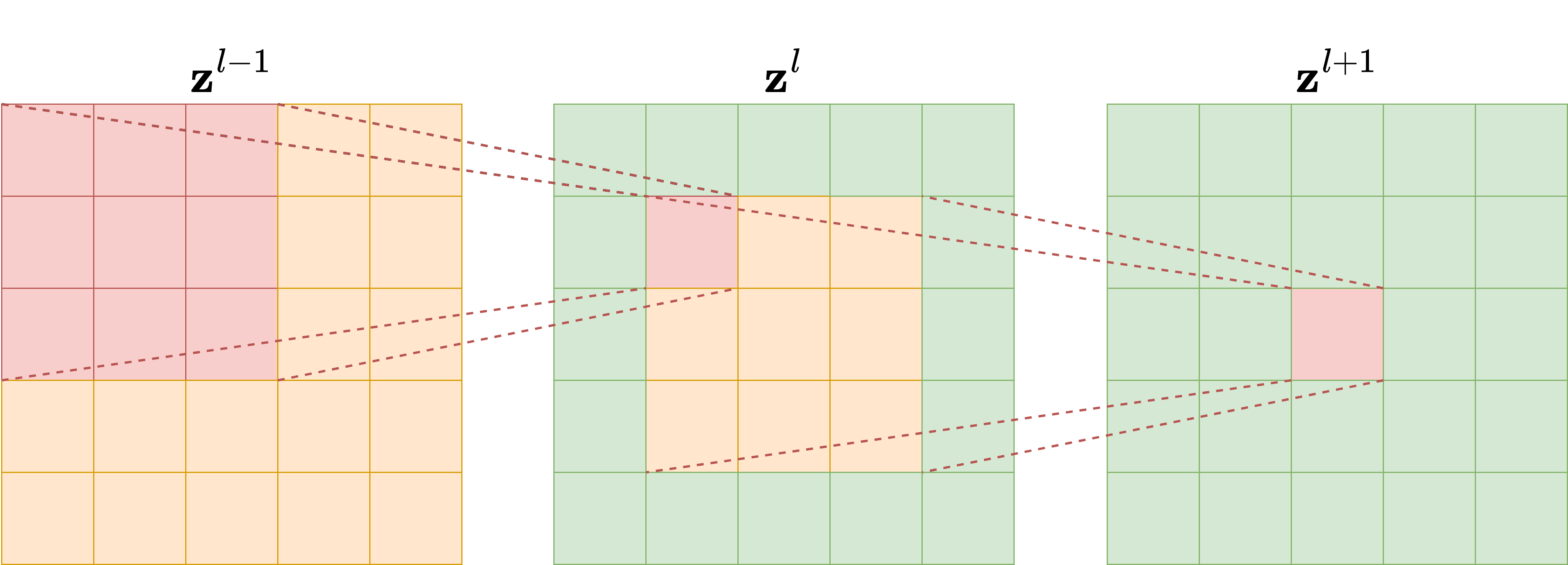
Fig. 10 Stacking local filters enlarges the region of input that can influence a feature. The count is a side length in each coordinate, rather than an area. Figure from Computational Imaging.#
With \(3\times3\) kernels, dilation one, and stride one, \(r_L=1+2L\). Three layers see a \(7\times7\) region, as in the denoising baseline. If the strides of four layers are \((1,2,1,2)\), the successive pairs \((r_\ell,j_\ell)\) are \((3,1)\), \((5,2)\), \((9,2)\), and \((13,4)\). The third layer adds four input pixels to the span because it operates on a grid already spaced by two. Pooling follows the same bookkeeping when treated as another local operation. In a network with multiple branches, the receptive field is the union of the fields of all incoming paths, rather than the count along an arbitrary single branch.
For generation the interpretation depends on the task. A discriminator with a small receptive field can assess local texture without checking global arrangement. A denoiser at high noise levels needs broad context because individual neighborhoods contain little identifiable signal. A decoder must organize long-range relationships while refining details. Downsampling is useful precisely because local operations on a coarse grid correspond to large regions of the original image.
Downsampling, Upsampling, and the Meaning of an Adjoint#
A feature hierarchy often halves height and width while increasing channels. A level with twice as many channels and half the resolution in each direction has about half as many scalar activations as the preceding level. This is a practical convention, not a theorem of optimal representation. Strided convolutions learn how to mix and subsample; average pooling applies a fixed local average; max pooling selects a local maximum and is nonlinear. Decimation can alias high-frequency structure, so a change of scale also changes which information is distinguishable.
The loss of information can be stated without appealing to visual intuition. If a linear downsampling map \(\boldsymbol{A}:\mathbb{R}^n\to\mathbb{R}^m\) has \(m<n\), the rank-nullity theorem gives a nonzero \(\boldsymbol{h}\) with \(\boldsymbol{A}\boldsymbol{h}=\boldsymbol{0}\). Hence \(\boldsymbol{A}\boldsymbol{x}=\boldsymbol{A}(\boldsymbol{x}+\boldsymbol{h})\). No decoder that sees only this observation can recover both inputs exactly. A learned decoder can exploit restrictions of the data distribution, but it cannot turn a noninjective operator into an inverse on the entire ambient space.
The expanding path of an encoder-decoder uses interpolation followed by convolution, or a learned transposed convolution. These operations need a precise interpretation.
Proposition 4 (A transposed convolution is an adjoint, not generally an inverse)
Represent a bias-free convolution on finite grids as a matrix \(\boldsymbol{A}\). Its Euclidean adjoint is the transpose \(\boldsymbol{A}^\top\), characterized by
For \(\ell(\boldsymbol{x})=\frac12\|\boldsymbol{A}\boldsymbol{x}-\boldsymbol{y}\|_2^2\), the gradient is \(\boldsymbol{A}^\top(\boldsymbol{A}\boldsymbol{x}-\boldsymbol{y})\). Exact reconstruction by transpose after encoding would require \(\boldsymbol{A}^\top\boldsymbol{A}=\boldsymbol{I}\), which is impossible when \(\boldsymbol{A}\) has fewer rows than columns.
Proof. Expanding the finite inner products and interchanging the two sums gives the adjoint identity. Differentiating the quadratic gives \(d\ell=(\boldsymbol{A}\boldsymbol{x}-\boldsymbol{y})^\top\boldsymbol{A}\,d\boldsymbol{x}\), hence the gradient formula. Applying transpose after the forward map gives \(\boldsymbol{A}^\top\boldsymbol{A}\boldsymbol{x}\), equal to every \(\boldsymbol{x}\) exactly when the product is the identity. If the map reduces dimension, its rank is less than \(n\), so that product cannot have rank \(n\).
In a generative decoder, a transposed convolution is usually an independently learned layer, not the transpose of a particular trained encoder layer. The name describes the connectivity pattern. Uneven overlap between its contributions can introduce spatial artifacts; resizing followed by a stride-one convolution is a useful alternative. Neither choice creates information from nothing: the output is determined by the code, skip features, conditioning variables, and learned weights.
Residual Learning and Two Kinds of Skip Connection#
A residual block computes \(\boldsymbol{h}_{out}=\boldsymbol{h}+F_\theta(\boldsymbol{h})\) when dimensions agree, or uses a learned projection on the skip branch when they do not. For image restoration, a related construction predicts a correction to the observed image. If \(\boldsymbol{Y}=\boldsymbol{X}+\sigma\boldsymbol{\varepsilon}\) and the network predicts \(\boldsymbol{r}(\boldsymbol{Y})\) with reconstruction \(\boldsymbol{Y}-\boldsymbol{r}(\boldsymbol{Y})\), squared-error regression gives
This follows immediately from Theorem 2 and linearity of conditional expectation. Predicting the residual and predicting the clean conditional mean are equivalent unrestricted problems. Their parameterizations and optimization behavior can differ. Residual learning does not prove that artifacts are independent of image content or that a model generalizes automatically to a new dataset.
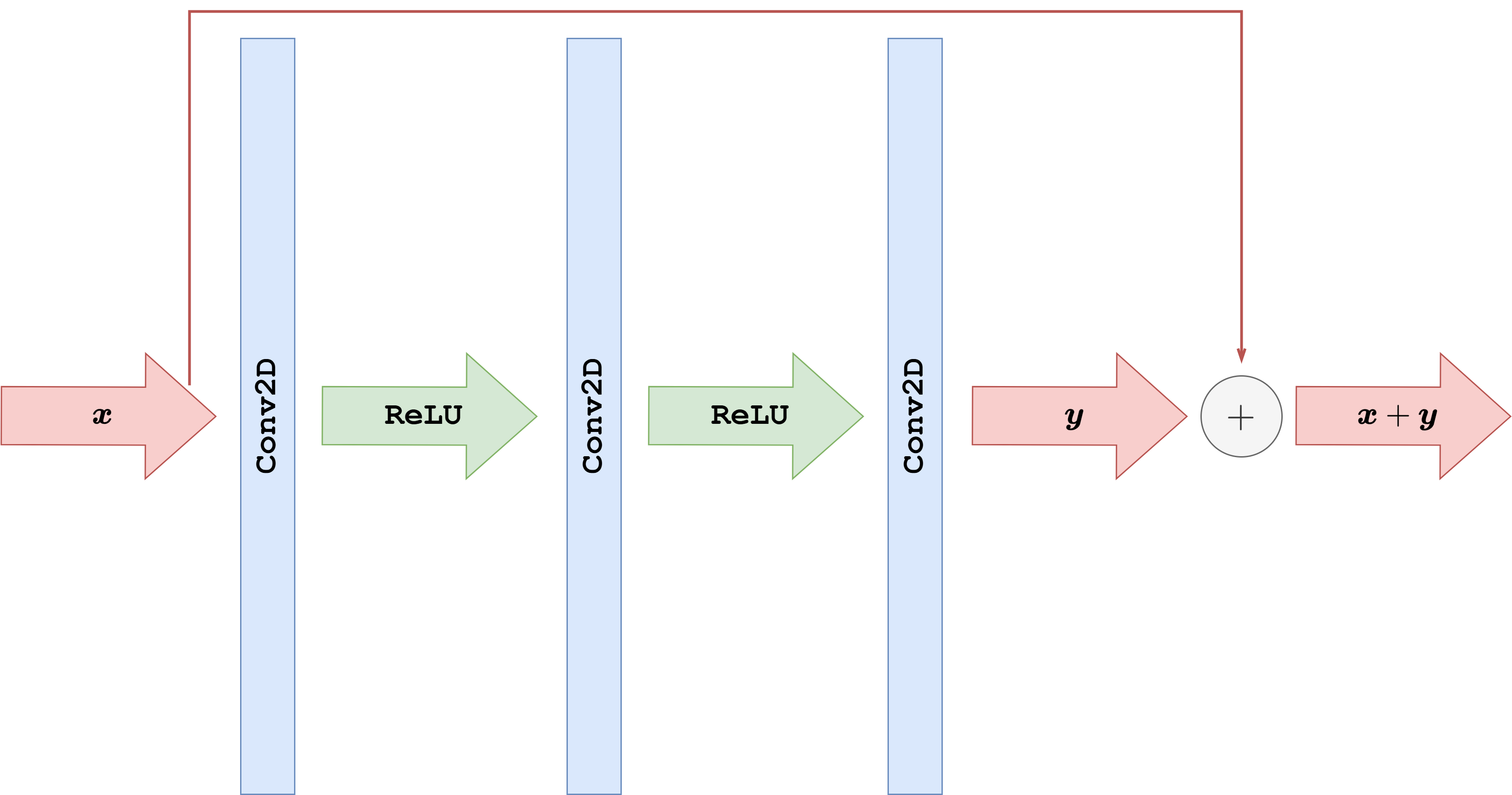
Fig. 11 A residual architecture provides a direct path for its input and learns a correction. The sign of that correction depends on whether the target is clean minus noisy or noisy minus clean. Figure from Computational Imaging.#
At a differentiability point, the block Jacobian is \(\boldsymbol{I}+\boldsymbol{J}_F\). Backpropagation therefore has a direct identity contribution. If \(\|\boldsymbol{J}_F\|_2\leq\rho<1\), the triangle inequality gives
The lower bound follows by the reverse triangle inequality and the upper bound by the ordinary triangle inequality. This is a local stability statement under an explicit hypothesis, not a guarantee that every residual network avoids vanishing or exploding gradients [HZRS16].
An encoder-decoder skip has a different purpose. It forwards a high-resolution feature tensor to a later decoder level, often by concatenation along channels. If each branch has \(C\) channels, addition returns \(C\) channels and requires matching channel semantics, while concatenation returns \(2C\) channels and lets a subsequent convolution learn the mixture. Both are called skips, but they route information differently.
The U-Net as a Multiscale Image-Valued Map#
A U-Net pairs a contracting path with an expanding path and joins corresponding resolution levels [RFB15]. The contracting path computes features with increasing spatial reach. The expanding path progressively restores the output grid. Encoder features remain available at each matching resolution, so the bottleneck need not carry every detail needed for localization. This makes the architecture useful when input and output share a coordinate system, as in denoising, score prediction, and velocity prediction.
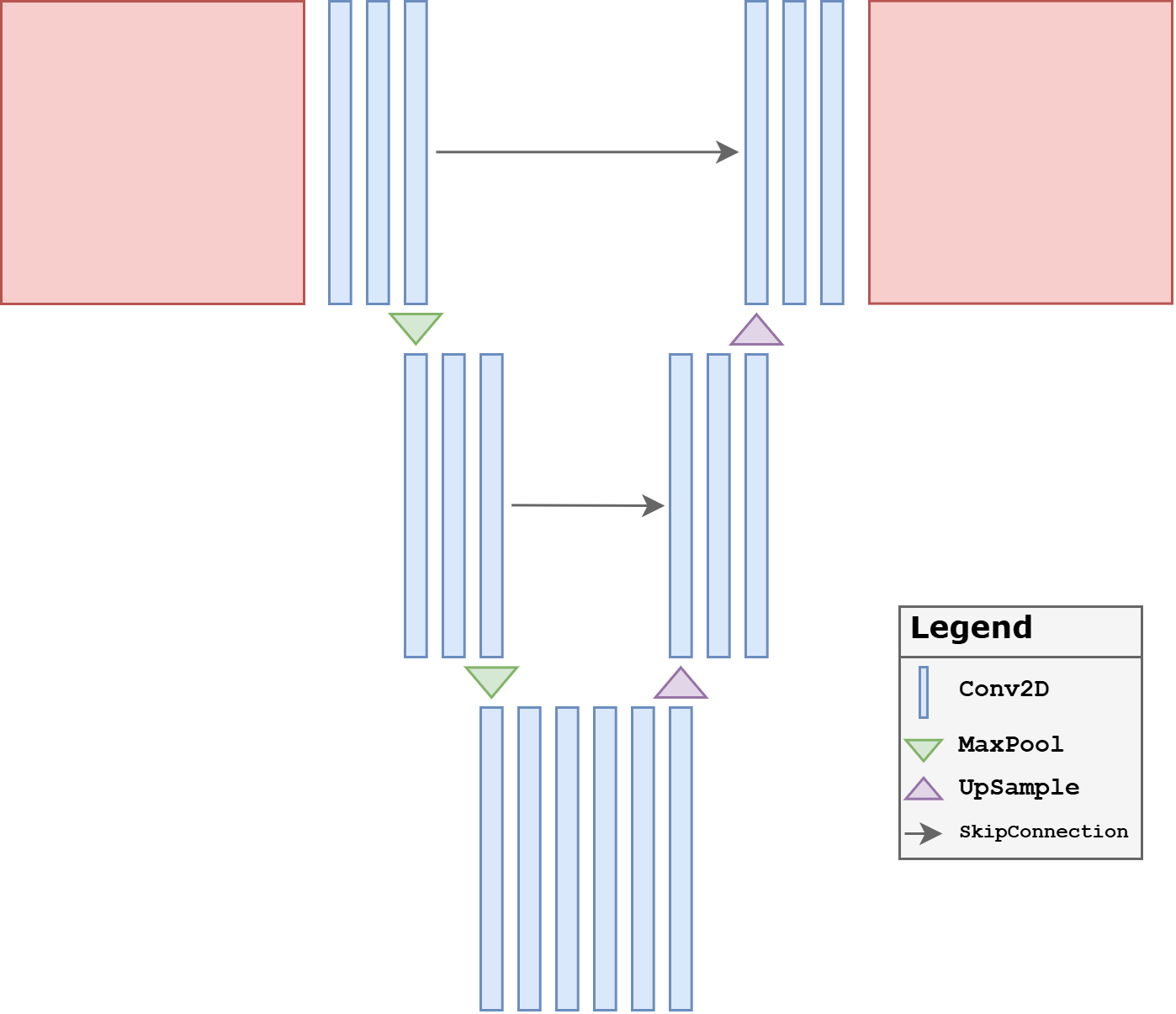
Fig. 12 The encoder supplies broad context; the decoder combines it with spatially detailed skip features. In a diffusion model the output is usually a noise or score estimate, rather than a segmentation map.#
For a small two-level example, a batch of grayscale \(32\times32\) images becomes a tensor of shape \((B,16,32,32)\) after the first block. A stride-two convolution gives \((B,32,16,16)\). After processing the bottleneck, interpolation restores \((B,32,32,32)\). Concatenating the first skip produces \((B,48,32,32)\), and a decoder block followed by a \(1\times1\) convolution returns \((B,1,32,32)\). Every concatenation must match height and width. Odd image sizes require an explicit resize or crop convention; assuming that every input size divides evenly is a frequent implementation error.
The U-Net is not information preserving in the sense of being invertible. Downsampling can discard information, activations can be noninjective, and the final projection can reduce channels. Its skips provide routes that help retain useful detail. During high-noise denoising they also carry noise, so the decoder must learn how much to use. The architecture supplies access to information; the objective determines whether that information is used appropriately.
Contrast this with a latent-variable autoencoder,
Here a bottleneck may be intentional: generation will later draw a latent code without access to an observed clean image. If a training-time decoder can bypass the code through unrestricted clean-image skips, its good reconstructions do not establish that the latent-only generation path works. A U-Net denoiser, by contrast, always receives its current noisy state during sampling. Its image skips are part of the available input, so their role is consistent between training and use.
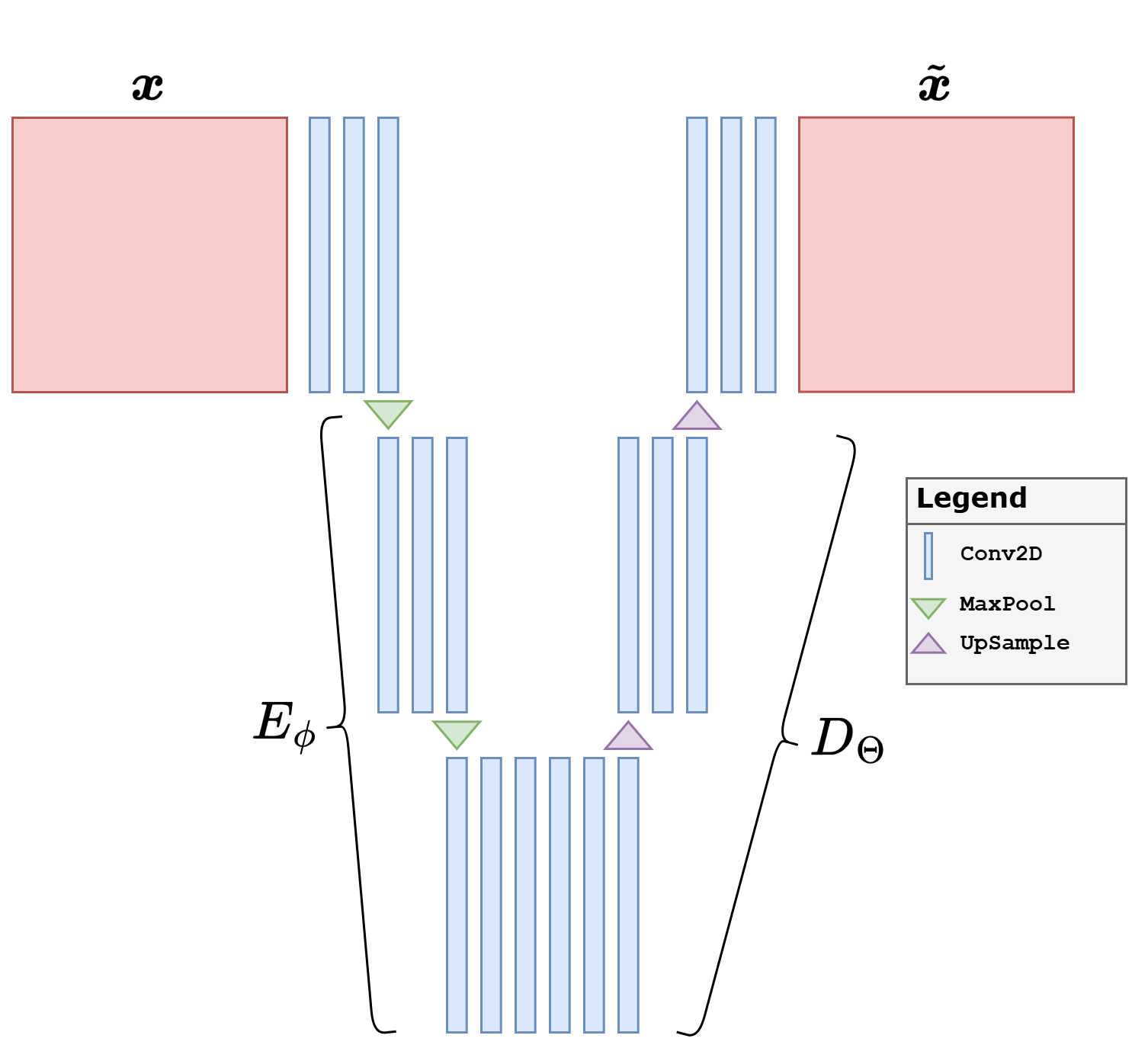
Fig. 13 A deterministic autoencoder reconstructs through a code. A prior over that code is an additional modeling ingredient, which will become central in the VAE chapter.#
Time and Other Conditioning Variables#
The map required by diffusion is \(\boldsymbol{\varepsilon}_\theta(\boldsymbol{x}_t,t)\), rather than one fixed denoiser applied identically at every noise level. The same observed value can have different interpretations at different noise levels. Flow matching similarly learns \(\boldsymbol{v}_\theta(\boldsymbol{x}_t,t)\). Thus time is part of the input to the statistical prediction problem. In a discrete diffusion implementation, integer step indices must be converted using the same convention during training and sampling.
A scalar time can be embedded into a feature vector, for example
An MLP transforms this vector into channelwise offsets or scales. A conditioned feature block may compute
The parameters are shared over spatial positions, so the conditioning modulates a feature field without assigning a separate time embedding to every pixel. Group normalization computes statistics within each sample and is convenient for small batches; batch normalization depends on batch statistics during training and running estimates during evaluation. Changing normalization can therefore change the predictor beyond its parameter count.
Class conditioning adds an embedding of a label. Text conditioning supplies a sequence of features that can interact with image features through cross-attention. We do not need a full transformer architecture here. The relevant distinction is whether conditioning is a global modulation or a content-dependent interaction. A bare convolutional network has the receptive-field limitation derived above; an attention layer can introduce direct interactions between distant positions, so the same local recurrence no longer describes the complete graph.
The compact implementation below makes time conditioning and the skip shapes explicit. It is a teaching backbone, not a trained generator. The sinusoidal embedding uses normalized times in \([0,1]\), and the last projection is linear because both noise and velocity targets can have either sign.
import math
import torch
from torch import nn
import torch.nn.functional as F

class TimeEmbedding(nn.Module):
    def __init__(self, width=32):
        super().__init__()
        self.register_buffer("frequencies", 2 * math.pi * 2.0 ** torch.arange(width // 2))
        self.projection = nn.Sequential(nn.Linear(width, width), nn.SiLU(), nn.Linear(width, width))

    def forward(self, time):
        phase = time[:, None] * self.frequencies[None, :]
        return self.projection(torch.cat([phase.sin(), phase.cos()], dim=1))

class ConditionalBlock(nn.Module):
    def __init__(self, in_channels, out_channels, time_width=32):
        super().__init__()
        self.conv1 = nn.Conv2d(in_channels, out_channels, 3, padding=1)
        self.norm = nn.GroupNorm(4, out_channels)
        self.modulation = nn.Linear(time_width, 2 * out_channels)
        self.conv2 = nn.Conv2d(out_channels, out_channels, 3, padding=1)
        self.skip = nn.Conv2d(in_channels, out_channels, 1) if in_channels != out_channels else nn.Identity()

    def forward(self, image, embedding):
        features = self.norm(self.conv1(image))
        scale, shift = self.modulation(embedding).chunk(2, dim=1)
        features = (1 + scale[:, :, None, None]) * features + shift[:, :, None, None]
        features = self.conv2(F.silu(features))
        return F.silu(features + self.skip(image))

class TinyConditionalUNet(nn.Module):
    def __init__(self):
        super().__init__()
        self.time = TimeEmbedding()
        self.encoder = ConditionalBlock(1, 16)
        self.down = nn.Conv2d(16, 32, 3, stride=2, padding=1)
        self.bottleneck = ConditionalBlock(32, 32)
        self.decoder = ConditionalBlock(48, 16)
        self.output = nn.Conv2d(16, 1, 1)

    def forward(self, image, time):
        embedding = self.time(time)
        skip = self.encoder(image, embedding)
        coarse = self.bottleneck(self.down(skip), embedding)
        up = F.interpolate(coarse, size=skip.shape[-2:], mode="bilinear", align_corners=False)
        return self.output(self.decoder(torch.cat([up, skip], dim=1), embedding))

torch.manual_seed(3)
model = TinyConditionalUNet()
image = torch.randn(2, 1, 32, 32)
time = torch.tensor([0.2, 0.8])
prediction = model(image, time)
print("Input/output shapes:", tuple(image.shape), tuple(prediction.shape))
print("Parameters:", sum(p.numel() for p in model.parameters()))
Input/output shapes: (2, 1, 32, 32) (2, 1, 32, 32)
Parameters: 42161
One architecture can now participate in two different statistical constructions. For diffusion, the input is \(\boldsymbol{x}_t=a_t\boldsymbol{x}_0+b_t\boldsymbol{\varepsilon}\) and the target can be \(\boldsymbol{\varepsilon}\). For a linear flow-matching path, the input is \((1-t)\boldsymbol{x}_0+t\boldsymbol{x}_1\) and the target is \(\boldsymbol{x}_1-\boldsymbol{x}_0\). An output tensor of the right shape is necessary in both cases, but shape alone does not determine its meaning. The distribution of input-target pairs defines the map being learned.
# A single diffusion-style regression step, using synthetic clean images.
torch.set_num_threads(2)
clean = torch.rand(2, 1, 32, 32)
time = torch.tensor([0.25, 0.75])
alpha = torch.exp(-2 * time)[:, None, None, None]
noise = torch.randn_like(clean)
noisy = alpha.sqrt() * clean + (1 - alpha).sqrt() * noise
optimizer = torch.optim.Adam(model.parameters(), lr=1e-3)
optimizer.zero_grad(set_to_none=True)
loss = F.mse_loss(model(noisy, time), noise)
loss.backward()
optimizer.step()
print("One noise-regression step:", float(loss.detach()))

# The same backbone also accepts odd image sizes without a skip mismatch.
with torch.no_grad():
    print("Odd-size output:", tuple(model(torch.randn(2, 1, 31, 29), time).shape))
One noise-regression step: 1.0711175203323364
Odd-size output: (2, 1, 31, 29)
This one-step example deliberately stops before proposing a generative sampler. A denoising loss only becomes a diffusion model after we specify the forward family, its reverse transition or score-based dynamics, and a terminal distribution. Likewise, velocity regression becomes a generator after we justify that its field transports the chosen source law. The architecture is now available for those arguments, but it does not replace them.
The mathematical background that follows introduces probability laws, conditional densities, and latent-variable constructions. The roles of the image networks can then be stated precisely: an encoder parameterizes inference, a decoder parameterizes an observation law, a discriminator compares populations, and a conditioned U-Net parameterizes a denoising or transport field. The implementation vocabulary remains shared even as the probability model changes [GBC16, PGM+19].