
Neural Networks as Trainable Maps for Imaging#
The introduction placed a probability distribution at the center of image generation. We now pause to understand the functions through which that distribution will be represented and learned. This is a useful pause for an audience trained in mathematics: the familiar objects are functions, compositions, derivatives, and optimization problems, while the unfamiliar part is often the precise role of a network inside a probabilistic construction. A decoder returns parameters of a conditional law. A discriminator returns a scalar test of two populations. A diffusion network returns an image-sized noise estimate. These are different maps, even when their implementations reuse the same convolutional blocks.
This chapter and the next form a background block intended for roughly two to three hours of teaching, including the small computational examples. We begin with images as elements of a finite-dimensional space and with the statistical meaning of learning a map. We then introduce differentiation, convolution, and the training loop. The next chapter develops receptive fields, multiscale architectures, U-Nets, and conditioning. The purpose throughout is to make the later generative constructions readable; classification benchmarks and architectural variants that do not serve that purpose can wait.
The imaging viewpoint follows the progression used in Computational Imaging: represent an image, learn a transformation, understand locality, and then introduce multiscale information flow. Here the destination changes. Restoration provides a controlled first example, and the same mathematics will later explain denoising score matching and flow matching.
Images, Tensors, and the Function We Want to Learn#
An image with \(C\) channels and spatial dimensions \(H\times W\) is an array \(\boldsymbol{x}\in\mathbb{R}^{C\times H\times W}\). By fixing an ordering of its entries we may identify it with a vector in \(\mathbb{R}^d\), where \(d=CHW\). Probability densities and Euclidean norms refer to this vector space; convolutions retain the array organization. These are two descriptions of the same object. The Frobenius norm of the array equals the Euclidean norm of its vectorization.
In code, a batch adds an index: a PyTorch tensor typically has shape \((B,C,H,W)\). The batch dimension is neither another spatial direction nor a learned feature channel. A feature tensor with 64 channels is also not a 64-color image: each channel is an intermediate scalar field produced by learned filters. Keeping these distinctions explicit prevents many apparent mathematical difficulties from becoming shape errors.
Intensity normalization is a change of coordinates with statistical consequences. An 8-bit image is discrete, with values in \(\{0,\ldots,255\}\). Dividing by 255 changes the scale but does not make its distribution continuous. When we use a Gaussian density on pixels, we adopt a continuous observation model, possibly after dequantization. When we use a Bernoulli likelihood, its exact sample space is binary. A soft grayscale target in a binary cross-entropy loss is a useful surrogate, but it is not literally a Bernoulli observation. This distinction will matter when we interpret the VAE objective.
Consider a clean random image \(\boldsymbol{X}\) and a corrupted observation \(\boldsymbol{Y}\). In an additive Gaussian example,
The network \(f_\theta\) maps an observation to a clean-image estimate. We choose it by minimizing a population risk
This expectation is over the joint law of clean images and corruptions. Training does not give access to the population expectation; it gives sample averages. Before discussing numerical optimization, it is worth identifying the mathematical target of this objective.
Theorem 2 (Squared-error regression is conditional expectation)
Let \(\boldsymbol{U}\in L^2(\Omega;\mathbb{R}^m)\) and let \(\boldsymbol{Y}\) be an observed random variable. For every measurable \(f\) with \(f(\boldsymbol{Y})\in L^2\), set \(\boldsymbol{m}(\boldsymbol{Y})=\mathbb{E}[\boldsymbol{U}|\boldsymbol{Y}]\). Then
Consequently, the unrestricted minimizer is the conditional mean, uniquely up to equality almost surely under the law of \(\boldsymbol{Y}\).
Proof. Write \(\boldsymbol{U}-f=(\boldsymbol{U}-\boldsymbol{m})+(\boldsymbol{m}-f)\) and expand the squared norm. The cross term vanishes because
The remaining two terms give the identity. The second is nonnegative and is zero exactly when \(f(\boldsymbol{Y})=\boldsymbol{m}(\boldsymbol{Y})\) almost surely.
The theorem explains both the strength and the limitation of a denoiser trained by mean squared error. It estimates a conditional average. If two sharp images are both plausible explanations of the same observation, their conditional mean can lie between them and appear smooth. Minimizing this loss does not mean drawing a random clean image from the conditional distribution. A neural network restricted to a finite architecture only approximates the unrestricted minimizer, and a finite optimization run introduces another approximation. We will reuse precisely this projection argument for noise prediction, score matching, and velocity regression.
Affine Maps, Nonlinear Features, and Differentiation#
A feedforward network is a composition. With \(\boldsymbol{h}_0=\boldsymbol{x}\), a hidden layer has the form
The parameter vector \(\theta\) collects all matrix and bias entries. The final layer is chosen for the object the network must return. A decoder may return a mean, a log-variance, or Bernoulli logits. A critic returns an unrestricted real number. A noise predictor and a velocity predictor return signed tensors. We should therefore not impose a sigmoid merely because the input happens to be an image.
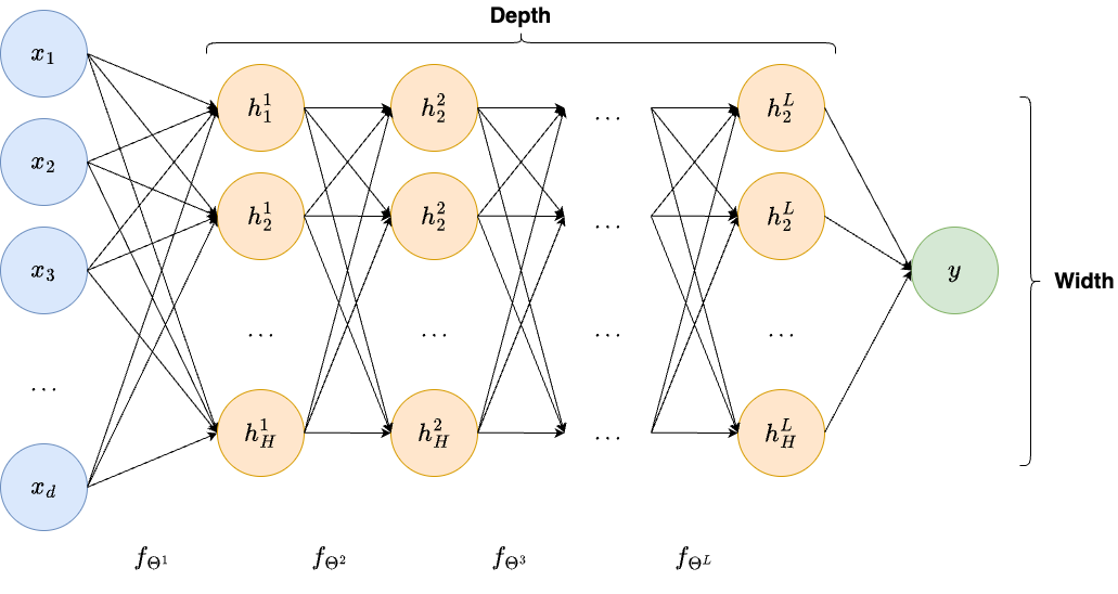
Fig. 7 An MLP composes affine transformations with pointwise nonlinearities. Convolutional architectures keep the composition principle while changing the linear operators.#
Without nonlinearities, two layers give \(\boldsymbol{W}_2(\boldsymbol{W}_1\boldsymbol{x}+\boldsymbol{b}_1)+\boldsymbol{b}_2\), another affine map. Nonlinearity is therefore essential for representing nonlinear image structure. ReLU, \(\sigma(a)=\max\{a,0\}\), is simple and 1-Lipschitz. SiLU, \(\sigma(a)=a/(1+e^{-a})\), is smooth and common in diffusion networks. Choosing an activation also chooses differentiability and stability properties; expressivity alone does not decide the architecture.
At this stage we do not need a universal approximation theorem. Existence of arbitrarily accurate approximants would not explain how many data are needed, how optimization finds parameters, or why spatial weight sharing is appropriate. We instead derive the operation that makes training possible: differentiation of a composition in reverse order [RHW86].
Proposition 1 (Backpropagation through affine and pointwise layers)
Let \(\ell\) be a scalar differentiable loss of the output, and suppose all activations are differentiable at the current preactivations. If \(\boldsymbol{g}_\ell=\nabla_{\boldsymbol{h}_\ell}\ell\), define
Then
Proof. The differential is \(d\boldsymbol{h}_\ell=\operatorname{diag}(\sigma_\ell'(\boldsymbol{a}_\ell))d\boldsymbol{a}_\ell\), and \(d\boldsymbol{a}_\ell=(d\boldsymbol{W}_\ell)\boldsymbol{h}_{\ell-1}+\boldsymbol{W}_\ell d\boldsymbol{h}_{\ell-1}+d\boldsymbol{b}_\ell\). Substituting in \(d\ell=\boldsymbol{g}_\ell^\top d\boldsymbol{h}_\ell\) gives
Identifying coefficients with respect to the Frobenius inner product for matrices and the Euclidean inner product for vectors gives the three formulas. Applying the last formula recursively propagates derivatives backward through the network.
At a ReLU kink the classical derivative does not exist; software adopts a specified subgradient convention, usually zero at the origin. The computation is differentiable almost everywhere, which is enough for the usual implementation but should not be confused with global smoothness. Automatic differentiation evaluates these chain-rule operations on a computational graph. It does not approximate the derivative by finite differences and does not differentiate the mathematical expectation automatically; we must justify any interchange of expectation and differentiation separately.
The same adjoint principle applies to convolutions and branching graphs. If a feature is used by two later computations, its derivative contributions add. If a layer is linear, its backward map is its adjoint. These observations will explain transposed convolutions and skip connections in the next chapter.
Convolution as a Structured Linear Operator#
A dense map from an RGB \(64\times64\) image to another vector of the same dimension would have \(12288^2=150994944\) weights before counting biases. It also assigns unrelated coefficients to the same local pattern appearing at two neighboring locations. A convolutional layer builds a more suitable hypothesis class by imposing locality and weight sharing [LBBH98].
Most deep-learning libraries implement cross-correlation and call it convolution. For stride one, one convenient convention is
Entries outside the image follow the padding convention. The kernel array \(\boldsymbol{K}\) is learned, while its pattern of reuse is fixed. In the classical mathematical definition of convolution the kernel is reversed; this difference changes the indexing convention, not the weight-sharing argument. In this course we use the library convention consistently.
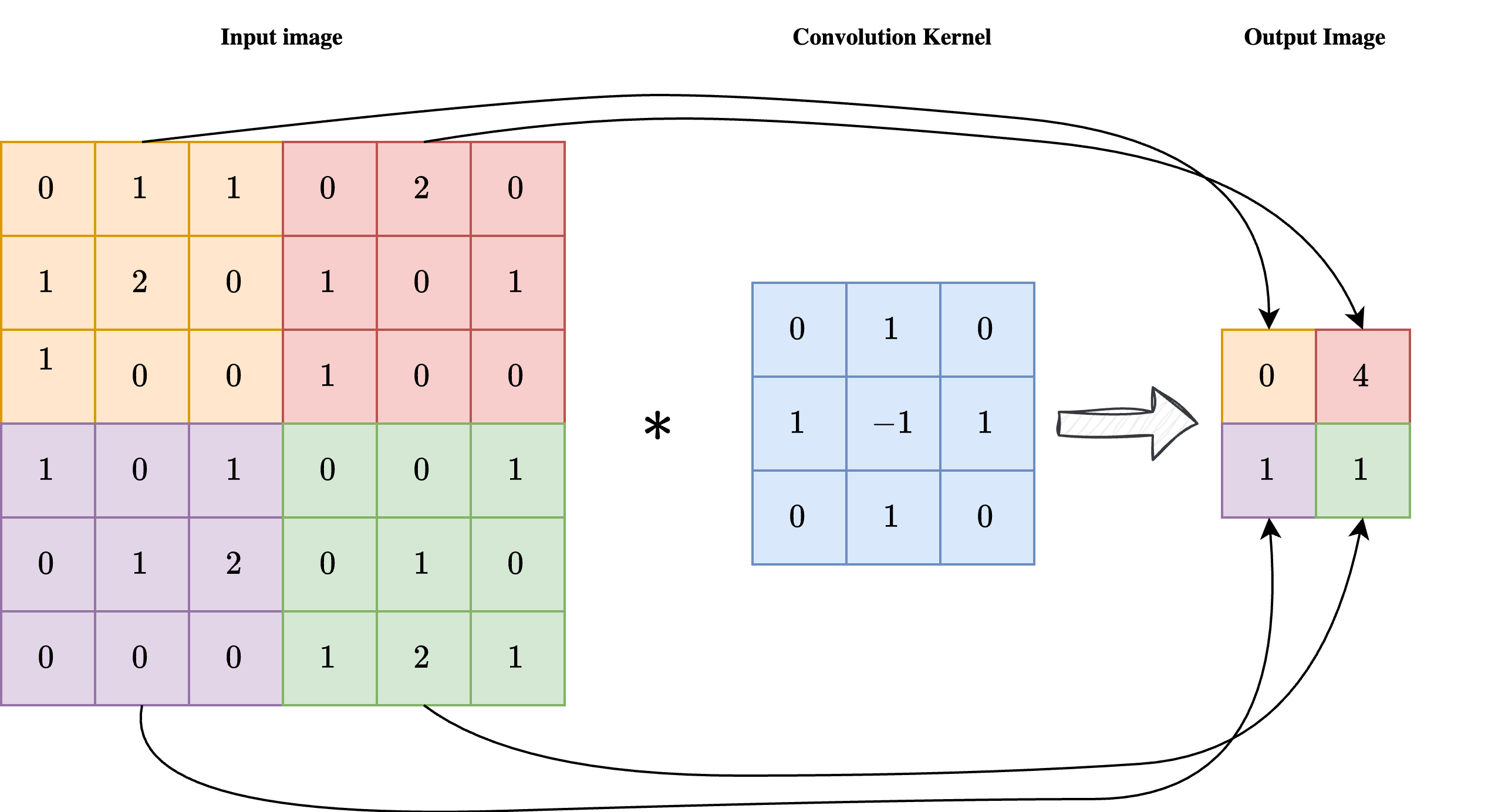
Fig. 8 A local kernel is reused across spatial positions. Figure adapted from the instructor’s Computational Imaging teaching material.#
With \(C_{out}\) output channels, a biased layer has \(C_{out}(C_{in}k_hk_w+1)\) parameters, independent of \(H\) and \(W\). A \(3\times3\) layer from 3 to 32 channels has 896 parameters. This reduction is not merely a memory saving: it assumes that a useful local transformation can be reused at different positions. The same feature extractor can consequently be used inside a VAE encoder, a GAN discriminator, or a denoising network, while the objective determines what features are useful.
Proposition 2 (Equivariance and its boundary conditions)
On the infinite grid \(\mathbb{Z}^2\), let \((T_{\boldsymbol{\tau}}\boldsymbol{x})_{c,\boldsymbol{i}}=x_{c,\boldsymbol{i}-\boldsymbol{\tau}}\). A stride-one convolution or cross-correlation with spatially constant bias satisfies
A pointwise activation commutes with the same translations, so a composition of such layers is equivariant as well.
Proof. For an output channel \(o\), write the finite kernel sum using offset \(\boldsymbol{r}\):
Also \(\sigma((T_{\boldsymbol{\tau}}\boldsymbol{x})_{c,\boldsymbol{i}})=\sigma(x_{c,\boldsymbol{i}-\boldsymbol{\tau}})=(T_{\boldsymbol{\tau}}\sigma(\boldsymbol{x}))_{c,\boldsymbol{i}}\). Commuting each layer through a composition proves the final statement.
This proposition does not imply exact equivariance for every practical image pipeline. Zero padding treats the boundary differently from the interior. Circular padding gives exact cyclic equivariance on a periodic grid. Downsampling with stride \(s\) preserves a corresponding relation for translations divisible by \(s\), but usually not for arbitrary one-pixel shifts. Equivariance also differs from invariance: in an image-to-image task, a shifted input should generally produce a shifted output, rather than the same output.
For one spatial coordinate, kernel size \(k\), dilation \(d\), padding \(p\) on each side, and stride \(s\), the output size is
The formula follows by counting valid starting positions of a window with span \(d(k-1)+1\). Apply it separately to height and width. A \(3\times3\) layer with stride one and padding one preserves size; with stride two it approximately halves it. Dilation increases the span of the kernel without adding coefficients. A convolutional block combines this linear map, an activation, and sometimes normalization. The resulting feature maps retain positions while changing the representation at each position.
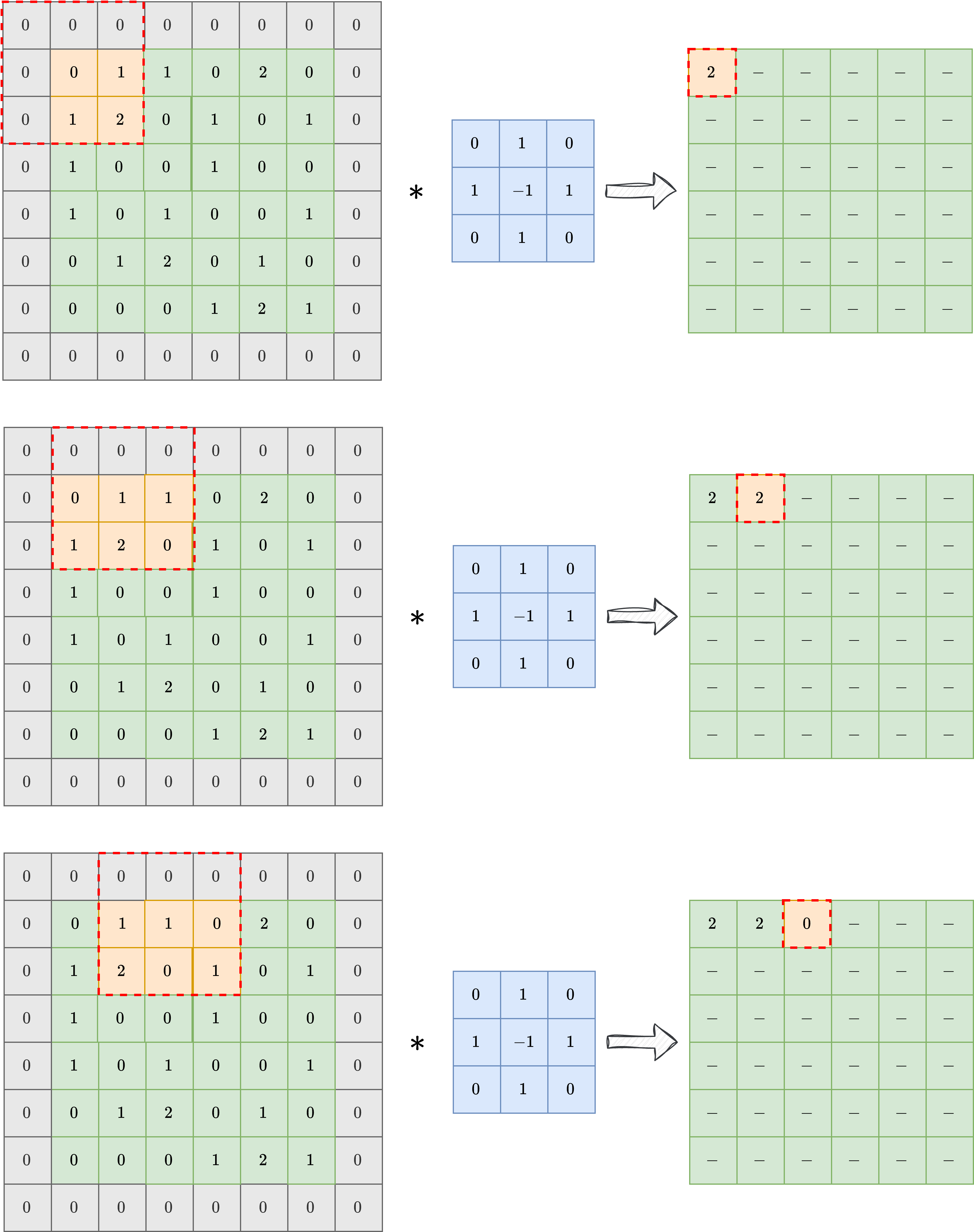
Fig. 9 Padding controls which neighborhoods are available at the boundary and changes output dimensions. Figure from Computational Imaging.#
From Population Risk to a Training Loop#
For independent clean training images \(\boldsymbol{x}^{(1)},\ldots,\boldsymbol{x}^{(n)}\), we can resample corruption during optimization and minimize an empirical expectation
Under a locally integrable domination assumption that permits differentiation under the expectation, sampling an index uniformly and an independent corruption gives an unbiased gradient estimator of \(R_n\). Indeed, linearity of expectation gives \(\mathbb{E}[\nabla_\theta\ell_i]=n^{-1}\sum_i\mathbb{E}_{\boldsymbol{\varepsilon}}[\nabla_\theta\ell_i]=\nabla_\theta R_n\). Averaging independent terms reduces variance. A minibatch update then has the form \(\theta_{k+1}=\theta_k-\eta_k\widehat{\nabla R_n}(\theta_k)\). Adam changes the update using running estimates of gradient moments [KB15]; it does not change which population problem the loss expresses.
There are three distinct questions. Can the architecture approximate the desired map? Can optimization fit that architecture to the training objective? Does the fitted map work on new images? Neither a small empirical loss nor a universal approximation statement answers all three. We therefore keep training and test images separate, control random seeds when comparing methods, and make preprocessing consistent. In later generative experiments, good reconstruction and good distribution matching will be distinct questions as well.
The following small experiment creates smooth synthetic images, corrupts them with Gaussian noise, and learns a denoiser. It needs no downloaded data and runs on CPU. The images are deliberately simple so that the role of the training objective stays visible. It is a regression baseline, not yet a procedure for generating new samples from the learned image distribution.
import torch
from torch import nn
import torch.nn.functional as F
import matplotlib.pyplot as plt

torch.manual_seed(7)
torch.set_num_threads(2)

def make_images(n, generator):
    axis = torch.linspace(-1, 1, 32)
    yy, xx = torch.meshgrid(axis, axis, indexing="ij")
    centers = 1.2 * torch.rand(n, 2, 1, 1, generator=generator) - 0.6
    widths = 0.12 + 0.25 * torch.rand(n, 2, 1, 1, generator=generator)
    image = torch.exp(-((xx - centers[:, 0]) / widths[:, 0]) ** 2
                      - ((yy - centers[:, 1]) / widths[:, 1]) ** 2)
    return image[:, None]

train_rng = torch.Generator().manual_seed(10)
test_rng = torch.Generator().manual_seed(20)
clean_train = make_images(256, train_rng)
clean_test = make_images(32, test_rng)
noisy_test = clean_test + 0.15 * torch.randn(clean_test.shape, generator=test_rng)

denoiser = nn.Sequential(
    nn.Conv2d(1, 16, 3, padding=1), nn.SiLU(),
    nn.Conv2d(16, 16, 3, padding=1), nn.SiLU(),
    nn.Conv2d(16, 1, 3, padding=1),
)
print("Input shape:", tuple(clean_train.shape))
print("Trainable parameters:", sum(p.numel() for p in denoiser.parameters()))
Input shape: (256, 1, 32, 32)
Trainable parameters: 2625
The last convolution is linear. For an additive-noise model, the optimal predictor is a real-valued conditional mean, and clipping it inside the training loss would impose another restriction. The network keeps the input resolution with padding one and sees only a \(7\times7\) neighborhood through its three \(3\times3\) layers. The next chapter derives this number and explains why it can become a limitation for realistic generative models.
optimizer = torch.optim.Adam(denoiser.parameters(), lr=2e-3)
loss_history = []
denoiser.train()
for step in range(100):
    indices = torch.randint(len(clean_train), (16,))
    target = clean_train[indices]
    noisy = target + 0.15 * torch.randn_like(target)
    optimizer.zero_grad(set_to_none=True)
    loss = F.mse_loss(denoiser(noisy), target)
    loss.backward()
    optimizer.step()
    loss_history.append(loss.item())

denoiser.eval()
with torch.no_grad():
    prediction = denoiser(noisy_test)
    input_mse = F.mse_loss(noisy_test, clean_test).item()
    output_mse = F.mse_loss(prediction, clean_test).item()
print(f"Held-out noisy MSE: {input_mse:.5f}")
print(f"Held-out denoised MSE: {output_mse:.5f}")

fig, axes = plt.subplots(1, 4, figsize=(12, 3))
for ax, image, title in zip(axes[:3], [clean_test[0, 0], noisy_test[0, 0], prediction[0, 0]],
                            ["Clean", "Noisy", "Predicted mean"]):
    ax.imshow(image, cmap="gray", vmin=0, vmax=1)
    ax.set_title(title)
    ax.axis("off")
axes[3].plot(loss_history)
axes[3].set(xlabel="Update", ylabel="Training MSE")
plt.tight_layout()
plt.show()
Held-out noisy MSE: 0.02259
Held-out denoised MSE: 0.00089
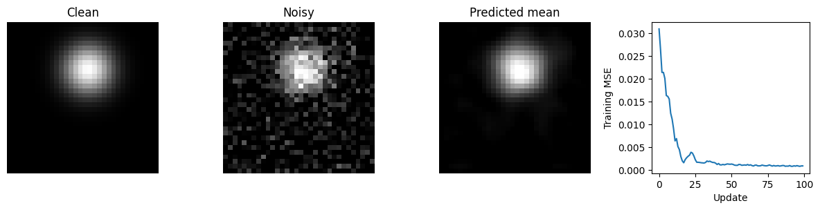
The code separates the mathematical roles cleanly. The synthetic image generator supplies training data; the Gaussian corruption supplies paired observations; the CNN parameterizes a map; automatic differentiation supplies a sample gradient; and Adam updates parameters. The network itself does not provide a prior over clean images. In diffusion, we will keep this regression mechanism but use a family of noise levels and a reverse dynamics to turn denoising information into generation. The next chapter explains the architecture needed when those corrections must reconcile fine texture with the organization of an entire image.