
Introduction to Generative Models#
A generative model is a probabilistic model for data. This sentence is short, but it contains the whole philosophy of the field. If images are viewed as random variables taking values in a high-dimensional space, then a generative model aims to describe the law according to which these images occur. Once such a law has been learned, new images can be sampled, partial information can be completed, missing content can be inferred, and prior knowledge can be injected into downstream tasks. In other words, generation is not only about synthesizing visually pleasing pictures. It is about learning a distribution rich enough to support reasoning.
Let \(\boldsymbol{x} \in \mathbb{R}^d\) denote an image and let \(p_{gt}(\boldsymbol{x})\) denote the unknown data-generating distribution. A learned model introduces a family \(\{p_\theta(\boldsymbol{x}) : \theta \in \Theta\}\) and tries to choose parameters \(\theta\) so that \(p_\theta\) is close to \(p_{gt}\). The central technical problem is that \(p_{gt}\) is never known analytically. We only observe samples \(\boldsymbol{x}^{(1)}, \ldots, \boldsymbol{x}^{(n)}\). Deep generative modeling is therefore the study of how to represent and fit complicated distributions using neural networks from finite data.
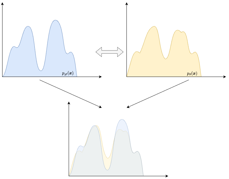
Fig. 3 A distributional representation of how deep generative model learns.#
Before we can talk about latent variables, variational bounds, or diffusion paths, we need a clear picture of the target problem itself. What does it mean to learn a distribution rather than a classifier? Why is image generation harder than label prediction? Which criteria distinguish model families at a high level? Those are the questions this chapter is meant to stabilize.
One reason this problem is harder than it may first appear is that high-dimensional image space is dominated by configurations that do not look like natural images at all. If one samples pixel values independently at random, the result is almost always meaningless noise. Natural images form a tiny, highly structured subset of the ambient space, with strong dependencies across locations, scales, and semantic content. A generative model is successful only when it captures these dependencies well enough that fresh samples fall near the same structured region as the data. The challenge is therefore geometric as much as statistical.
A useful way to summarize this idea is through the manifold hypothesis. The hypothesis says, informally, that although images are represented as very high-dimensional vectors, realistic images do not occupy that entire ambient space uniformly. Instead, they concentrate near a much smaller structured set. In other words, the number of raw coordinates needed to store an image is huge, but the number of truly independent factors needed to describe plausible images is often much smaller. Pose, lighting, object identity, background, texture, viewpoint, and style may vary, but they vary in correlated and constrained ways rather than arbitrarily.
This point is easier to understand with a simple contrast. A \(128 \times 128\) RGB image lives in an ambient space of dimension \(128 \cdot 128 \cdot 3 = 49152\). From a purely mathematical perspective, any point in \(\mathbb{R}^{49152}\) is an image-sized vector. But almost all such vectors look like nonsense to a human observer. They do not correspond to natural faces, animals, landscapes, or medical scans. The manifold hypothesis says that the visually meaningful data live near a much thinner region inside this enormous space. The figure below should be read in exactly that spirit: the cloud of realistic samples occupies a narrow structured set embedded inside a much larger ambient world.
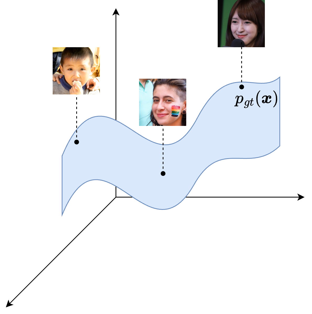
Fig. 4 The manifold hypothesis: samples from \(p_{gt}\) are distributed over a low-dimensional manifold embedded in \(\mathbb{R}^n\).#
It is important not to interpret this picture too literally. Real datasets are noisy, multimodal, and imperfect. The data do not usually lie on one clean mathematical manifold in the strict differential-geometric sense. The hypothesis should instead be understood as a modeling intuition: natural data occupy a highly constrained subset of image space, and this subset has far more structure than arbitrary pixel noise. That is already enough to motivate why generation is difficult. A successful model must learn not only which local textures are plausible, but also which global configurations of those textures can coexist.
This is also why latent variables become so natural later in the course. If images are controlled by a smaller collection of hidden explanatory factors, then it makes sense to search for a lower-dimensional representation that organizes those factors. VAEs do this through latent codes, GANs through a learned generator acting on simple noise, diffusion models through trajectories that stay close to the data manifold while denoising, and flow matching through learned transport fields. The exact machinery changes, but the geometric motivation is the same: realistic data are structured, concentrated, and far from uniform in ambient space.
This is also the right place to state an important philosophical point for the course. A generative model is not merely a machine for producing visually plausible outputs. It is a hypothesis about how data are organized. When we choose latent variables, adversarial critics, denoising paths, or transport fields, we are choosing not only an optimization objective but also a language for describing image distributions. Different model families correspond to different languages.
Generative Versus Discriminative Learning#
Discriminative models aim at conditional tasks such as predicting a label \(y\) from an image \(\boldsymbol{x}\). In probabilistic language, they approximate objects like \(p(y | \boldsymbol{x})\) or decision rules derived from it. Generative models target \(p(\boldsymbol{x})\) itself, or a joint distribution \(p(\boldsymbol{x}, \boldsymbol{z})\) involving hidden variables. This difference changes the geometry of the task. The image space is enormous, multimodal, and structured. Modeling its full law is more ambitious than solving a supervised prediction problem, but it also provides more flexibility.
A deep generative model is therefore not merely a classical generative model with a large parameter count. The adjective deep signals that the parameterization is compositional and learned by neural networks. The decoder of a VAE, the generator of a GAN, the score network of a diffusion model, and the velocity field of a flow matching model are all examples of neural parameterizations that transform a simple distribution into a complicated one.
It is often helpful to contrast the information demanded by the two paradigms. A discriminative classifier may succeed even if it learns only the features necessary to separate categories. It does not need to know how to generate the full image, nor how likely one background texture is relative to another when both correspond to the same label. A generative model, by contrast, must account for the whole observation. It must model nuisance variation, texture, shape, layout, and all the dependencies that make an image look coherent. This is why generative learning is typically harder, but also why it can be more powerful once successful.
For students who are less familiar with the machine-learning distinction, one simple metaphor can help. A discriminative model acts like an examiner who sees an answer sheet and decides which class it belongs to. A generative model acts like an author who must know how to produce a plausible answer sheet in the first place. The second task contains much richer structural information.
Why Likelihood Matters, and Why It Is Not the Whole Story#
If a model has a tractable density \(p_\theta(\boldsymbol{x})\), a natural learning principle is maximum likelihood: \(\theta^\star \in \arg\max_\theta \sum_{i=1}^n \log p_\theta(\boldsymbol{x}^{(i)})\). This objective has a clear statistical interpretation. Under standard assumptions, maximizing empirical log-likelihood amounts to minimizing the Kullback-Leibler divergence from the data distribution to the model family up to an additive constant. The next theorem makes this precise.
Theorem 1 (Maximum likelihood and forward Kullback-Leibler divergence)
Let \(p_{gt}\) be the true data distribution and let \(p_\theta\) be any model distribution such that \(\log p_\theta(\boldsymbol{x})\) is integrable under \(p_{gt}\). Then
Consequently, minimizing \(\operatorname{KL}(p_{gt} \| p_\theta)\) over \(\theta\) is equivalent to maximizing the expected log-likelihood under the data distribution.
Proof. By definition,
Splitting the logarithm gives
The first term does not depend on \(\theta\), so the minimizer of the divergence coincides with the maximizer of the second term. Replacing the population expectation with the empirical average yields the usual maximum likelihood estimator.
The previous argument is elegant, but in deep generative modeling exact likelihood is often unavailable or inconvenient. This is why different model families choose different compromises. Variational autoencoders keep a likelihood but optimize a lower bound because exact inference over latent variables is hard. GANs abandon explicit likelihood and train through adversarial discrimination. Diffusion models recover tractable objectives by decomposing generation into many small denoising steps. Flow matching learns vector fields that transport a simple distribution to the data distribution along a chosen probability path.
This variety of strategies is one of the reasons the field can feel fragmented at first. Students often ask whether VAEs, GANs, and diffusion models are competitors, unrelated inventions, or successive improvements of one universal idea. The right answer is more subtle. They are all trying to approximate the unknown data distribution, but they do so by making different tradeoffs between tractable probability, optimization stability, sample quality, and computational cost. A VAE gives us a transparent probabilistic story and amortized inference, but may blur samples. A GAN may produce sharp outputs, but its optimization is delicate and its density is implicit. A diffusion model is often stable and high quality, but sampling may be slow. Flow matching tries to retain the continuous-time transport viewpoint while simplifying training.
Once these tradeoffs are visible, the course becomes easier to navigate. One is not memorizing isolated acronyms, but studying different answers to the same foundational problem.
A First Taxonomy#
A first useful classification is to ask two questions. First, what probabilistic object is the model trying to represent? Second, how directly can we evaluate or manipulate that distribution? These questions lead to a taxonomy that is not perfect, but is extremely useful for orientation.
A central distinction is between explicit and implicit generative models. An explicit model is one in which the probability law is written down directly enough that likelihood, or at least a closely related probabilistic quantity, plays a central role in training. This does not necessarily mean that every computation is easy. It means the model is trying to describe a probability distribution in an overt probabilistic language. A VAE is explicit in this sense: it specifies a joint model \(p_\theta(\boldsymbol{x}, \boldsymbol{z}) = p_\theta(\boldsymbol{x} | \boldsymbol{z}) p(\boldsymbol{z})\), even though the marginal likelihood \(p_\theta(\boldsymbol{x}) = \int p_\theta(\boldsymbol{x} | \boldsymbol{z}) p(\boldsymbol{z}) \, d\boldsymbol{z}\) is usually intractable and must be handled through variational inference. Diffusion models are also explicit in spirit: they define a probabilistic forward corruption process and derive a principled training objective from that construction, even if the final implementation looks like denoising regression.
An implicit model, by contrast, is easy to sample from but does not provide a tractable density formula for an image. A GAN is the canonical example. One samples a latent noise vector, pushes it through the generator, and obtains an image. The induced distribution exists mathematically, but it is not available in a form that makes direct likelihood evaluation practical. Training therefore proceeds indirectly, through an adversarial critic rather than through explicit density computation.
A second axis concerns the role of latent structure. Some models use a single latent code, as in a VAE or a GAN. Others use an extended latent trajectory, as in diffusion models, where the hidden variables are the progressively corrupted states \(\boldsymbol{x}_1, \ldots, \boldsymbol{x}_T\). Flow matching sits nearby conceptually, but emphasizes a continuous transport field rather than a stochastic reverse chain. So one should not think only in terms of whether a model has a latent variable, but also in terms of what kind of latent mechanism it uses: a compact code, a long path, or a continuous flow.
Putting these axes together gives a more explicit map. VAEs are explicit probabilistic models with latent variables and approximate inference. GANs are implicit generative models with easy sampling and adversarial training. Diffusion models are explicit path-based probabilistic models whose training emerges from noising and denoising. Flow matching models are transport-based generative models that learn a deterministic velocity field and are best understood through continuous probability evolution rather than direct density evaluation. The labels are different, but the real value of the taxonomy is that it tells us what each family is choosing to make easy and what each family is choosing to make hard.
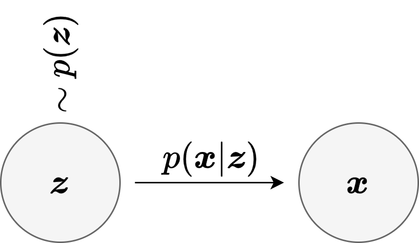
Fig. 5 The latent-variable viewpoint is one of the recurring conceptual templates of the course.#
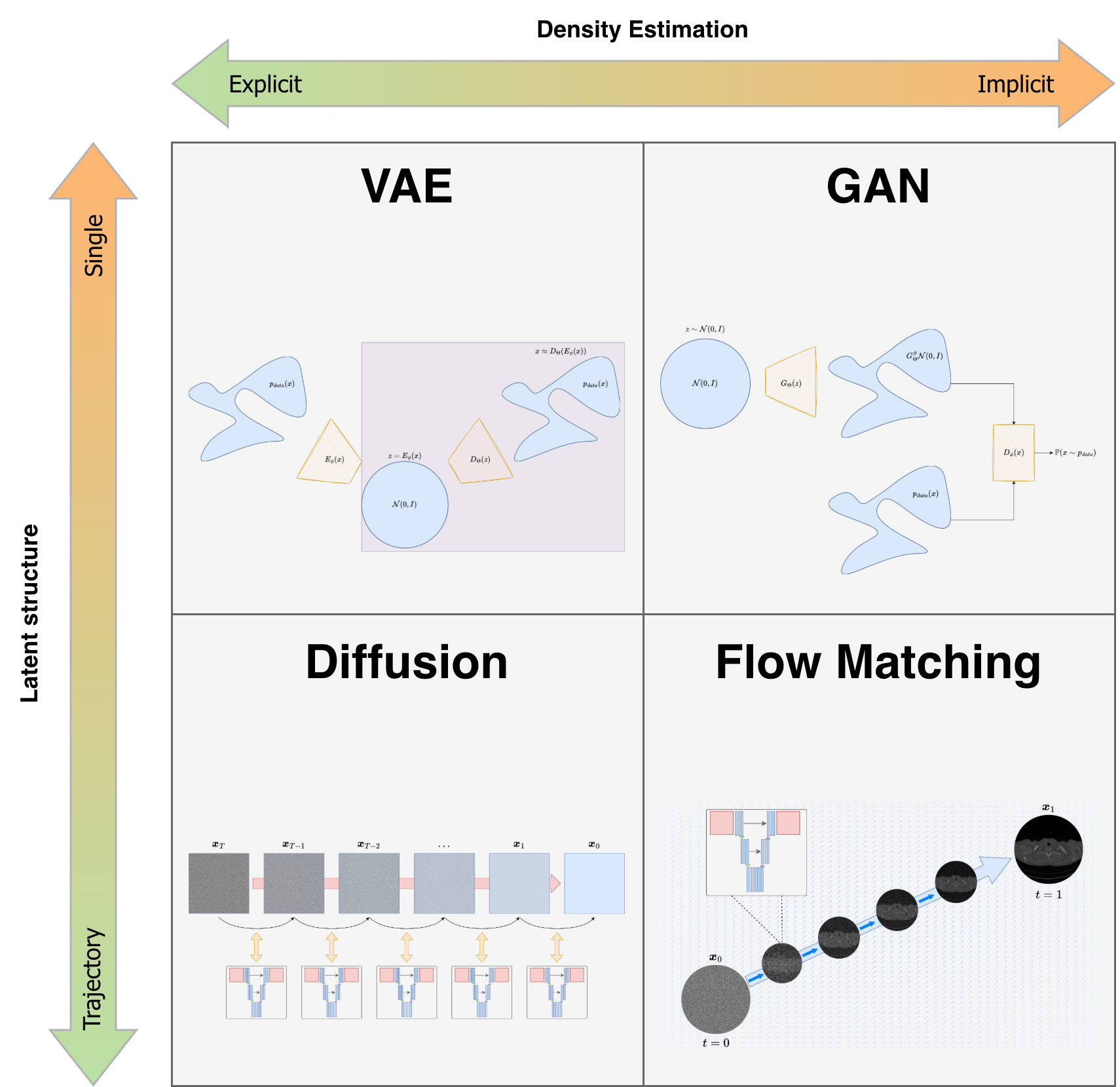
Fig. 6 A visual taxonomy of the main model families discussed in the course, organized by probabilistic representation and training strategy.#
It is also worth emphasizing that the taxonomy is not rigid. Many important modern systems are hybrids. Latent diffusion models combine autoencoding ideas with diffusion in latent space. Conditional GANs and conditional diffusion models add side information and no longer model only a plain marginal distribution. Normalizing flows provide exact likelihoods, so they are explicit models, but they are also continuous transport models. Some recent systems even mix autoregressive, latent, and diffusion-like components inside one pipeline.
For this reason, the taxonomy should be used as a reading tool rather than as a bureaucracy. When encountering a new paper, it is often enough to ask a short sequence of questions. Is the model explicit or implicit? If explicit, is the likelihood tractable, approximated, or only indirectly optimized? If implicit, what critic or matching principle supplies the training signal? Does the model use a compact latent code, a stochastic path, or a deterministic flow? Is training likelihood-based, adversarial, denoising-based, or transport-based? How is sampling actually performed in practice?
If a student can answer those questions for a new model, then the landscape stops looking like a list of fashionable acronyms and starts looking like a structured design space. That shift in viewpoint is one of the main goals of the early part of the course.
If these questions can be answered for a new paper, then the student has already understood the architecture of the field at a meaningful level.
For students who are less comfortable with the formalism, it is helpful to keep an intuitive image in mind. A generative model is an engine that starts from simple randomness and shapes it until it looks like structured data. The technical challenge is to decide how this shaping should be parameterized and how the parameters can be learned from examples. Everything in the rest of the course can be read as a refinement of this simple idea. Classical references that support the broad statistical viewpoint include [Bis06], while the modern deep learning context is discussed in [GBC16].