Cross-Domain End-to-End Reconstruction#
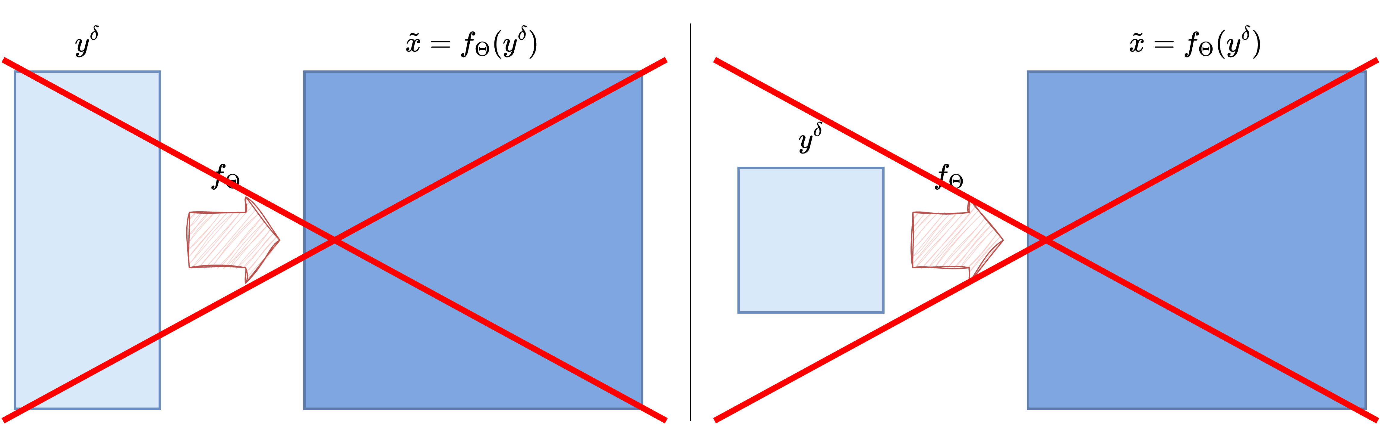
Despite the impressive performance (in terms of both reconstruction quality and efficiency) often achieved by convolution-based neural networks, their direct application in practice can be limited by a crucial constraint: their inherent structure typically requires the input data and the output solution to have matching dimensions. They struggle to process data where the dimensionality of the input datum \(y\) differs significantly from the dimensionality of the desired solution \(x\).
Consider, for example, the popular UNet architecture. Due to its symmetric encoding-decoding structure, the dimensionality of the model’s input remains unchanged at the output. This poses a challenge in applications such as Computed Tomography (CT) or Super-Resolution (SR), where the domain (and thus, often the dimensionality and structure) of the measured datum \(y\) is inherently different from the domain of the desired solution image \(x\).
Resizing?#
A seemingly straightforward solution to this limitation is to resize the input datum \(y\) so that its dimensions match the expected dimensions of the reconstruction \(x\). This could be achieved using functions like Resize() from the torchvision package. While this modification allows a model like UNet to technically process the mapping from the resized \(y\) to \(x\), this approach has generally been shown to be ineffective in practice for many inverse problems.
Indeed, convolution-based end-to-end models suffer from another limitation stemming from their core properties of locality and translation invariance (as discussed in a previous chapter). When information pertaining to the solution \(x\) gets spread widely across the measurement \(y\) (for instance, when the value of a pixel in \(x\) influences many, potentially spatially distant, pixels in \(y\)), convolutional filters struggle to accurately reconstruct the solution. The local receptive field of convolutions cannot easily capture these non-local dependencies, even if the input and output shapes are forced to match via resizing.
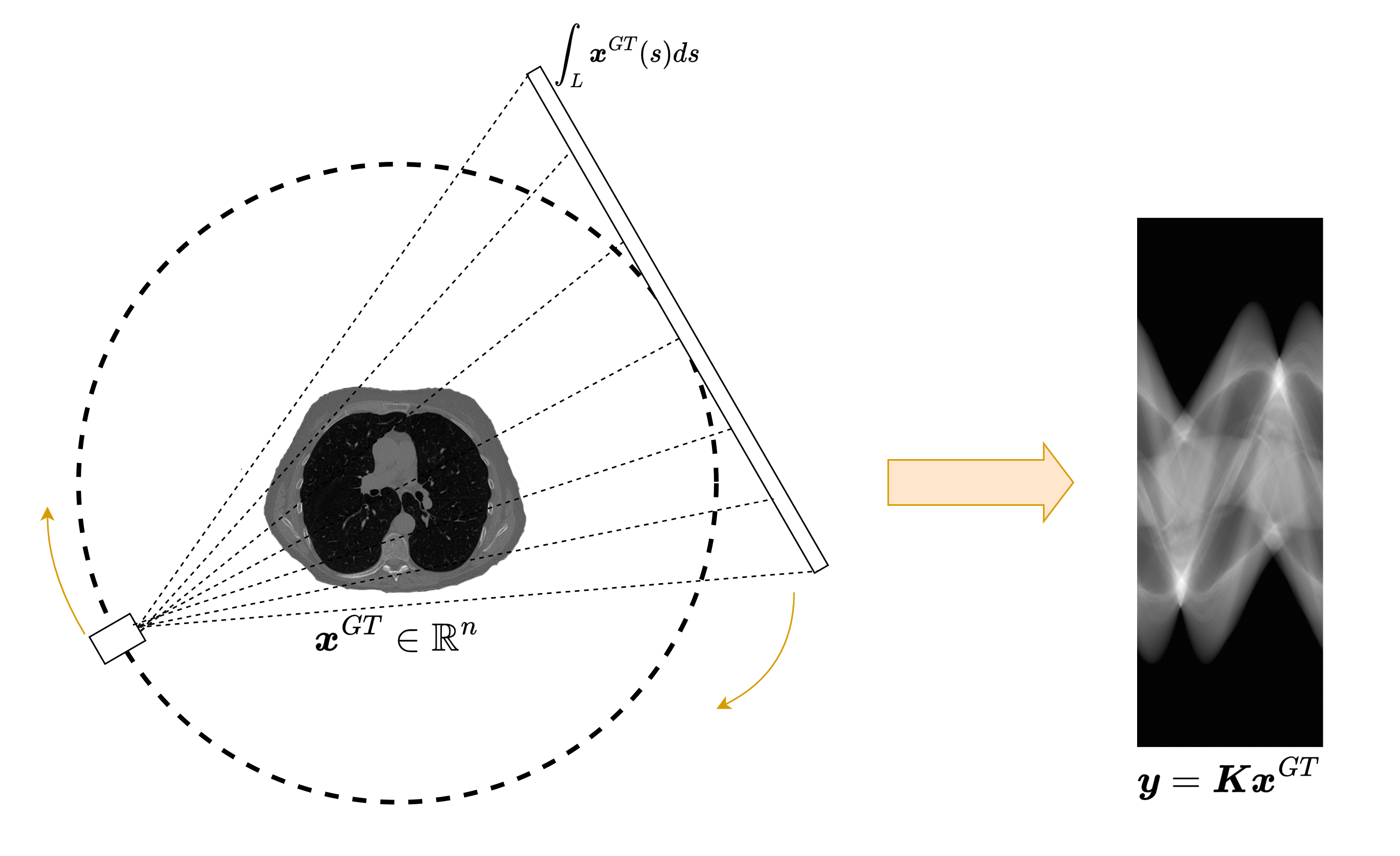
Consider the Computed Tomography (CT) inverse problem as an example. Here, the ground truth image \(x_{GT}\) is processed by the CT forward projection operator \(K\) to obtain a measurement \(y = Kx_{GT}\) called a sinogram. Each pixel \(y_{i, j}\) in the sinogram represents the line integral of \(x_{GT}\) along a specific path (e.g., line \(j\) at projection angle \(i\)). Clearly, not only are the shapes of \(x_{GT}\) (a 2D or 3D spatial image) and \(y\) (a sinogram with dimensions like number of angles \(\times\) number of detector bins, e.g., \((n_\alpha, n_d)\)) generally different, but locality is also lost. Each point in the sinogram \(y\) depends on multiple, potentially distant, pixels in the original image \(x_{GT}\). Consequently, a standard convolution-based model applied directly to the sinogram (even if resized) will likely be ineffective at reconstructing \(x_{GT}\).
Pre-processing#
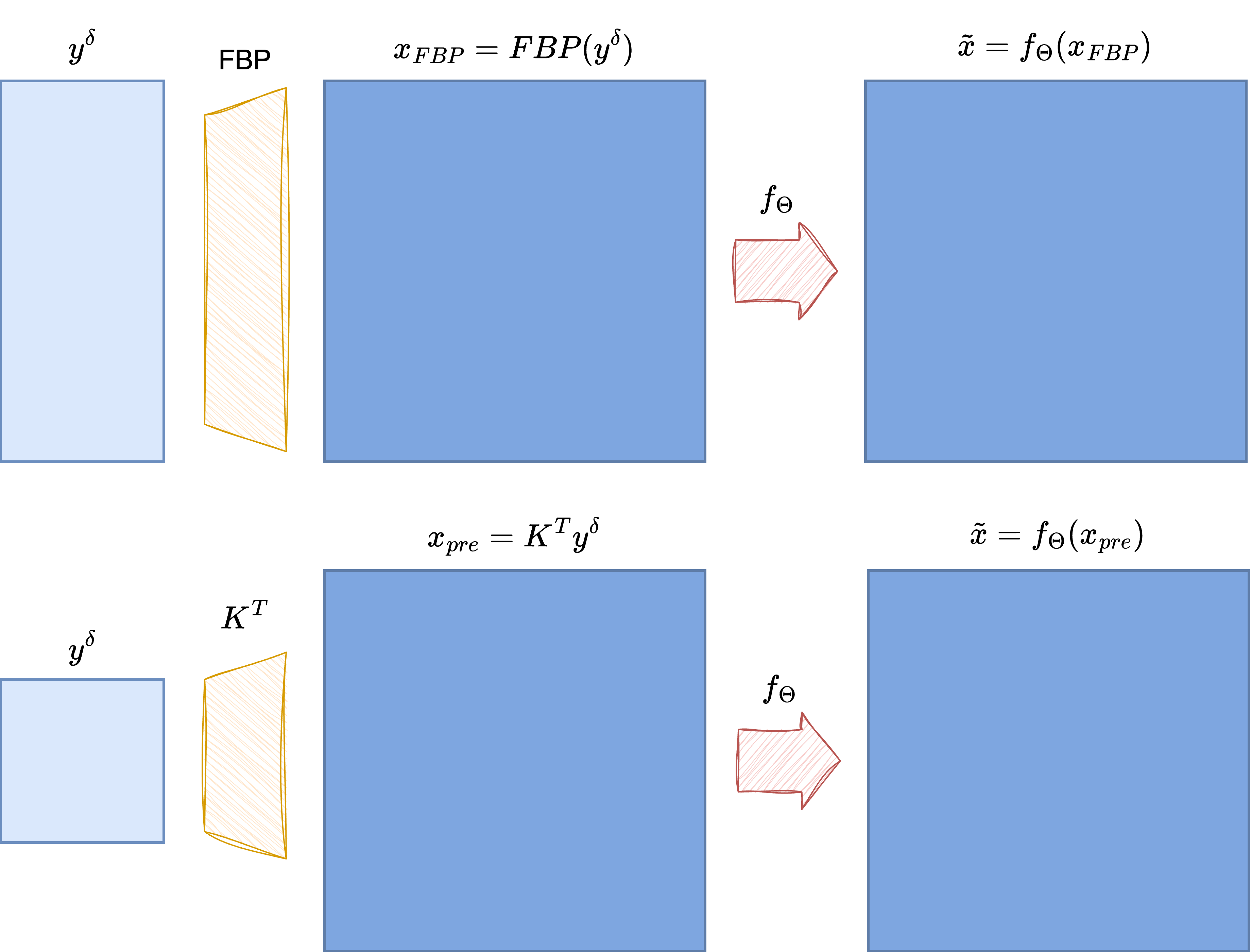
A classical and more robust solution to handle domain mismatch is to introduce a pre-processing step. The core idea is to apply an initial, often simple, reconstruction algorithm that maps the measurement \(y\) back into the domain of the solution \(x\), producing a coarse or approximate reconstruction \(\tilde{x}\). The quality of this initial reconstruction \(\tilde{x}\) is not the primary concern; its main purpose is to bridge the domain gap, providing an input that has the correct dimensionality and spatial structure for the subsequent neural network. The network then acts essentially as a post-processing or refinement layer, taking the coarse estimate \(\tilde{x}\) and producing the final, higher-quality reconstruction.
To minimize computational overhead and avoid potential bottlenecks, this initial approximation step should ideally be very fast. A classic approach is to use the transposed forward operator \(K^T\) (often related to back-projection in problems like CT) as a simple mapping:
Clearly, \(\tilde{x}\) will generally be a low-quality image, as \(K^T\) maps \(y\) back to the image domain without explicitly optimizing for reconstruction fidelity. However, this transformation is often computationally inexpensive, making it suitable for this pre-processing role. It stands to reason that if a better initial reconstruction \(\tilde{x}\) could be obtained efficiently (without significantly increasing computational time), the subsequent neural network might achieve a better final result, thereby increasing the overall effectiveness of the pipeline.
For this reason, more advanced pre-processing techniques have been developed, particularly in recent years. These methods are typically task-specific, as they often need to exploit the specific mathematical properties of the forward operator \(K\) to yield a higher-quality initial estimate than simple transposition or back-projection. In the following sections, we might discuss specific pre-processing approaches for common inverse problems like CT and SR. For other inverse problems where specialized pre-processing methods are not readily available, recall that using the transposed operator \(K^T\) always provides a basic, universally applicable pre-processing option.
A full pipeline to train end-to-end cross-domain UNet#
#-----------------
# This is just for rendering on the website
import os
import sys
import glob
sys.path.append("..")
#-----------------

from IPPy import operators, utilities, metrics, models
from IPPy.nn import trainer, losses

import torch
from torch import nn

from torch.utils.data import Dataset
from torchvision import transforms
from PIL import Image
import numpy as np

# Set device
device = utilities.get_device()

# Define model
model = models.UNet(ch_in=1,
                    ch_out=1,
                    middle_ch=[64, 128, 256],
                    n_layers_per_block=2,
                    down_layers=("ResDownBlock", "ResDownBlock"),
                    up_layers=("ResUpBlock", "ResUpBlock"),
                    final_activation=None).to(device)

# Define dataset class
class MayoDataset(Dataset):
    def __init__(self, data_path, data_shape):
        super().__init__()

        self.data_path = data_path
        self.data_shape = data_shape

        # We expect data_path to be like "./data/Mayo/train" or "./data/Mayo/test"
        self.fname_list = glob.glob(f"{data_path}/*/*.png")

    def __len__(self):
        return len(self.fname_list)

    def __getitem__(self, idx):
        # Load the idx's image from fname_list
        img_path = self.fname_list[idx]

         # To load the image as grey-scale
        x = Image.open(img_path).convert("L")

        # Convert to numpy array -> (512, 512)
        x = np.array(x)

        # Convert to pytorch tensor -> (1, 512, 512) <-> (c, n_x, n_y)
        x = torch.tensor(x).unsqueeze(0)

        # Resize to the required shape
        x = transforms.Resize(self.data_shape)(x) # (1, n_x, n_y)

        # Normalize in [0, 1] range
        x = (x - x.min()) / (x.max() - x.min())

        return x

# --- Load data
train_data = MayoDataset("../data/Mayo/train", data_shape=256)
train_loader = torch.utils.data.DataLoader(train_data, batch_size=4, shuffle=True)

# Define CTProjector operator
K = operators.CTProjector(
    img_shape=(256, 256),
    angles=np.linspace(0, np.pi, 60),
    det_size=512,
    geometry="parallel",
)

# --- Parameters
n_epochs = 0

loss_fn = losses.MixedLoss(
    (nn.MSELoss(), losses.SSIMLoss(), losses.FourierLoss()),
    (1, 0.1, 0.1),)
optimizer = torch.optim.Adam(params=model.parameters(), lr=1e-4)

# Cycle over the epochs
for epoch in range(n_epochs):

    # Cycle over the batches with tqdm
    epoch_loss = 0.0
    ssim_loss = 0.0
    for t, x in enumerate(train_loader):
        # Send x and y to device
        x = x.to(device)

        with torch.no_grad():
            # Compute associated y_delta
            y = K(x)
            y_delta = y + utilities.gaussian_noise(y, noise_level=0.01)

            # --- PREPROCESSING
            x_FBP = K.FBP(y_delta)

        # zero the parameter gradients
        optimizer.zero_grad()

        # forward + backward + optimize
        x_pred = model(x_FBP)
        loss = loss_fn(x_pred, x)
        loss.backward()
        optimizer.step()

        # update loss
        epoch_loss += loss.item()
        ssim_loss += metrics.SSIM(x_pred.cpu().detach(), x.cpu().detach())

        # Update tqdm bar
        print(
            {
                "Loss": f"{epoch_loss / (t + 1):.4f}",
                "SSIM": f"{ssim_loss / (t + 1):.4f}",
            }
        )

    # Save model every 5 epochs (overwrite)
    if (epoch + 1) % 5 == 0:
        # Save model state
        trainer.save(model, weights_path="../weights/CTUNet")
CUDA not available. CTProjector will use CPU.
Attempting to create ASTRA projector type: 'linear' for 'parallel' geometry...
Successfully created ASTRA projector type: 'linear'
CTProjector initialized. Geometry: parallel. Using GPU: False. FBP Algorithm: FBP