Introduction to Generative Models for Image Synthesis#
Generative models are a fundamental class of machine learning models that aim to learn the distribution of data in order to generate new, realistic samples. In the context of image processing, they allow us to synthesize novel images that are visually indistinguishable from real ones, by capturing the underlying data distribution of natural images.
While discriminative models focus on modeling the conditional probability \(p(y \mid x)\) — that is, predicting a label \(y\) given an input \(x\) — generative models try to model the full data distribution \(p(x)\), or more generally, the joint distribution \(p(x, y)\).
Why Generative Models?#
The ability to sample from a learned distribution has profound implications. Generative models can be used for:
Data augmentation: synthesize new examples to train better classifiers
Image denoising: estimate clean images from noisy ones
Inpainting: fill in missing parts of an image
Super-resolution: generate high-resolution images from low-resolution inputs
Compression: learn a compact latent representation of images
Creative applications: generate art, faces, textures, and more
In this chapter, we lay the foundation for understanding one of the most powerful classes of generative models today: diffusion models. But before diving into those, we start by exploring the general landscape of generative modeling.
The General Objective#
Let \(x \in \mathbb{R}^d\) denote an image (flattened to a vector), and let \(p_{\text{data}}(x)\) be the unknown data distribution. Our goal is to learn a model \(p_\theta(x)\), parameterized by \(\theta\), that approximates \(p_{\text{data}}(x)\).
The standard training objective is the maximum likelihood estimation (MLE):
Equivalently, this corresponds to minimizing the Kullback–Leibler (KL) divergence between the true data distribution and the model distribution:
The lower the KL divergence, the closer our model distribution is to the true one.
However, this framework depends on the ability to evaluate or estimate \(\log p_\theta(x)\), which is not always feasible. This leads to different classes of models, depending on how they approach this problem.
Categories of Generative Models#
We can divide generative models into different categories based on their modeling approach:
Latent Variable Models#
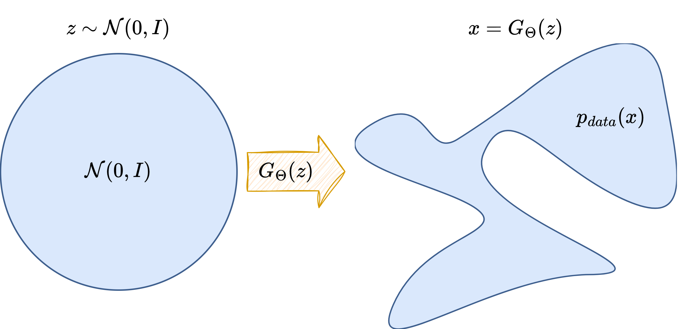
Latent variable models assume that observed data \(x\) is generated from some latent variable \(z\), typically sampled from a simple distribution such as a Gaussian:
Here, \(G_\theta\) is a neural network called the generator, mapping the latent space to the data space.
Two popular examples of this family are:
Variational Autoencoders (VAEs)
Generative Adversarial Networks (GANs)
We will now give a brief overview of both.
Variational Autoencoders (VAEs)#
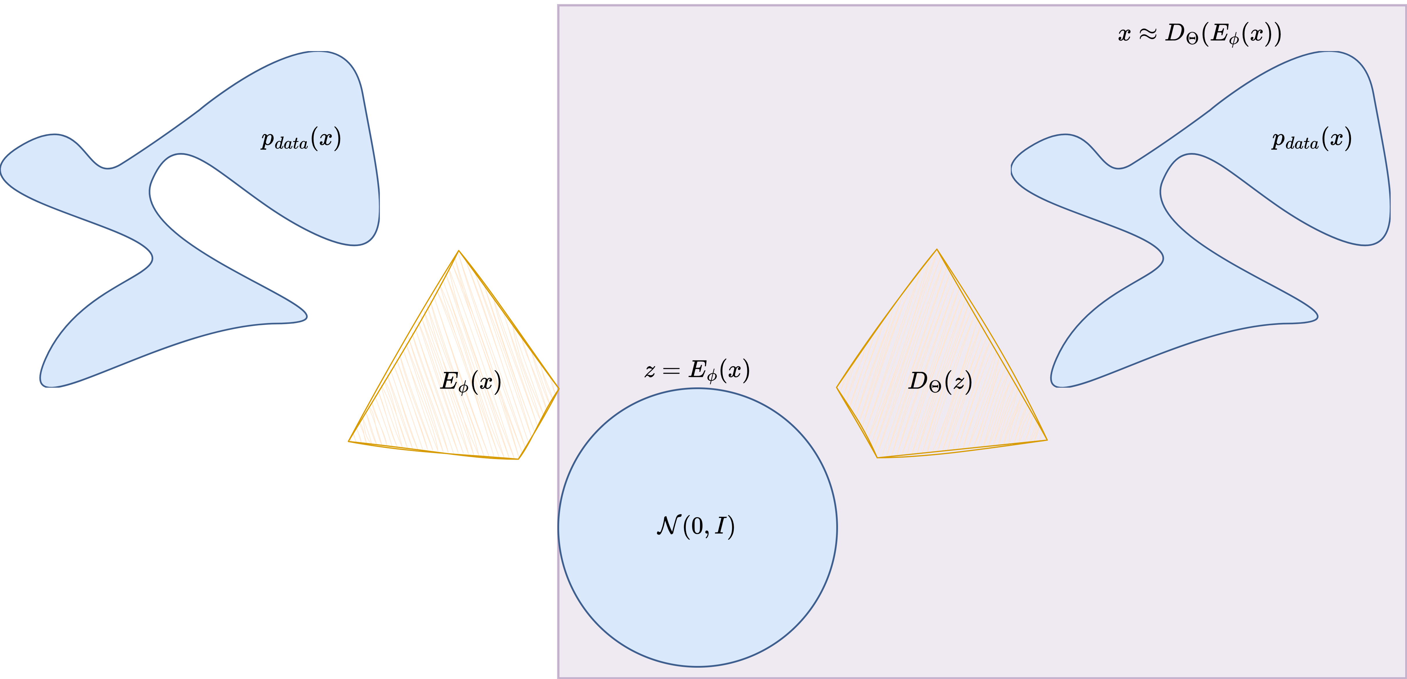
A VAE introduces an encoder \(q_\phi(z \mid x)\) and a decoder \(p_\theta(x \mid z)\). The encoder maps an image to a distribution over the latent space, and the decoder maps latent samples back to images.
The training objective maximizes a lower bound on the log-likelihood, known as the Evidence Lower BOund (ELBO):
The first term is a reconstruction term; the second is a regularization term that keeps \(q_\phi(z \mid x)\) close to the prior.
Pros:
Probabilistic interpretation
Well-defined log-likelihood
Cons:
Often produces blurry samples
Generative Adversarial Networks (GANs)#
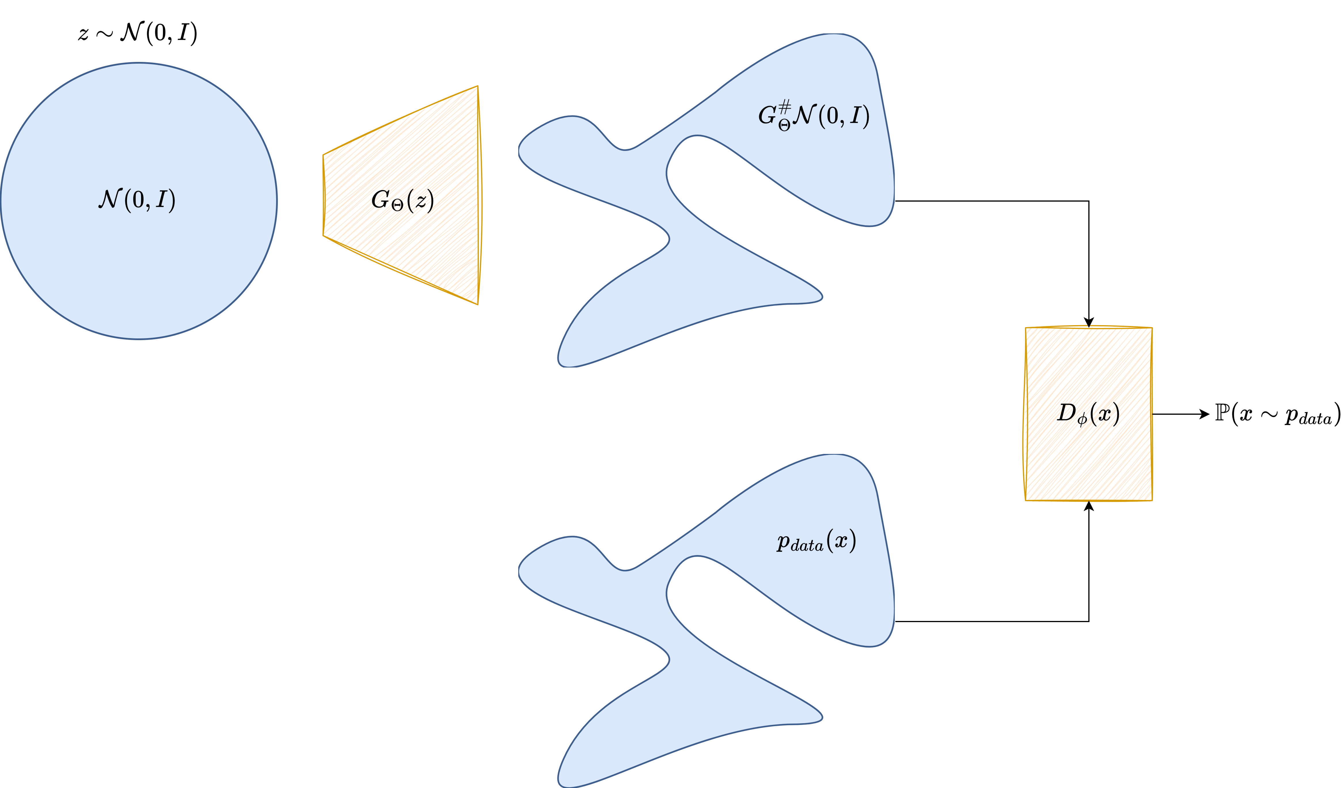
GANs are trained using an adversarial process between a generator \(G_\theta(z)\) and a discriminator \(D_\psi(x)\):
The generator maps latent variables \(z \sim p(z)\) to images
The discriminator tries to distinguish real images from generated ones
The training objective is a minimax game:
GANs are powerful but notoriously unstable during training. They do not model \(p(x)\) explicitly and can suffer from mode collapse.
A Minimal PyTorch Example: Latent Generator#
Here is a simple implementation of a generator network in PyTorch:
import torch
import torch.nn as nn

class SimpleGenerator(nn.Module):
    def __init__(self, latent_dim=100, image_shape=(1, 28, 28)):
        super().__init__()
        self.model = nn.Sequential(
            nn.Linear(latent_dim, 256),
            nn.ReLU(),
            nn.Linear(256, 512),
            nn.ReLU(),
            nn.Linear(512, int(torch.prod(torch.tensor(image_shape)))),
            nn.Tanh()  # Output in [-1, 1]
        )
        self.image_shape = image_shape

    def forward(self, z):
        img = self.model(z)
        return img.view(z.size(0), *self.image_shape)

# Sample usage
latent_dim = 100
generator = SimpleGenerator(latent_dim)
z = torch.randn(16, latent_dim)
generated_images = generator(z)
print(generated_images.shape)  # e.g., (16, 1, 28, 28)
torch.Size([16, 1, 28, 28])
Autoregressive and Flow-Based Models#
In addition to latent-variable models, other popular approaches include:
Autoregressive models: model \(p(x)\) as a product of conditionals, e.g., PixelCNN:
\[ p(x) = \prod_{i=1}^n p(x_i | x_{< i}), \]These are exact but slow to sample from.
Normalizing Flows: invertible neural networks that transform a simple distribution into a complex one using a series of bijections. The change-of-variable formula is used to compute:
Fast inference and exact likelihood, but limited expressivity compared to GANs.
Limitations of Existing Models#
While each approach has its advantages, there are also drawbacks:
VAEs struggle with image sharpness
GANs are unstable and lack a tractable likelihood
Autoregressive models are slow to sample from
Flows require architectural constraints to maintain invertibility
This motivates the development of diffusion models, which offer:
High-quality image synthesis
Stable training
A well-grounded probabilistic framework
Preview: What Are Diffusion Models?#
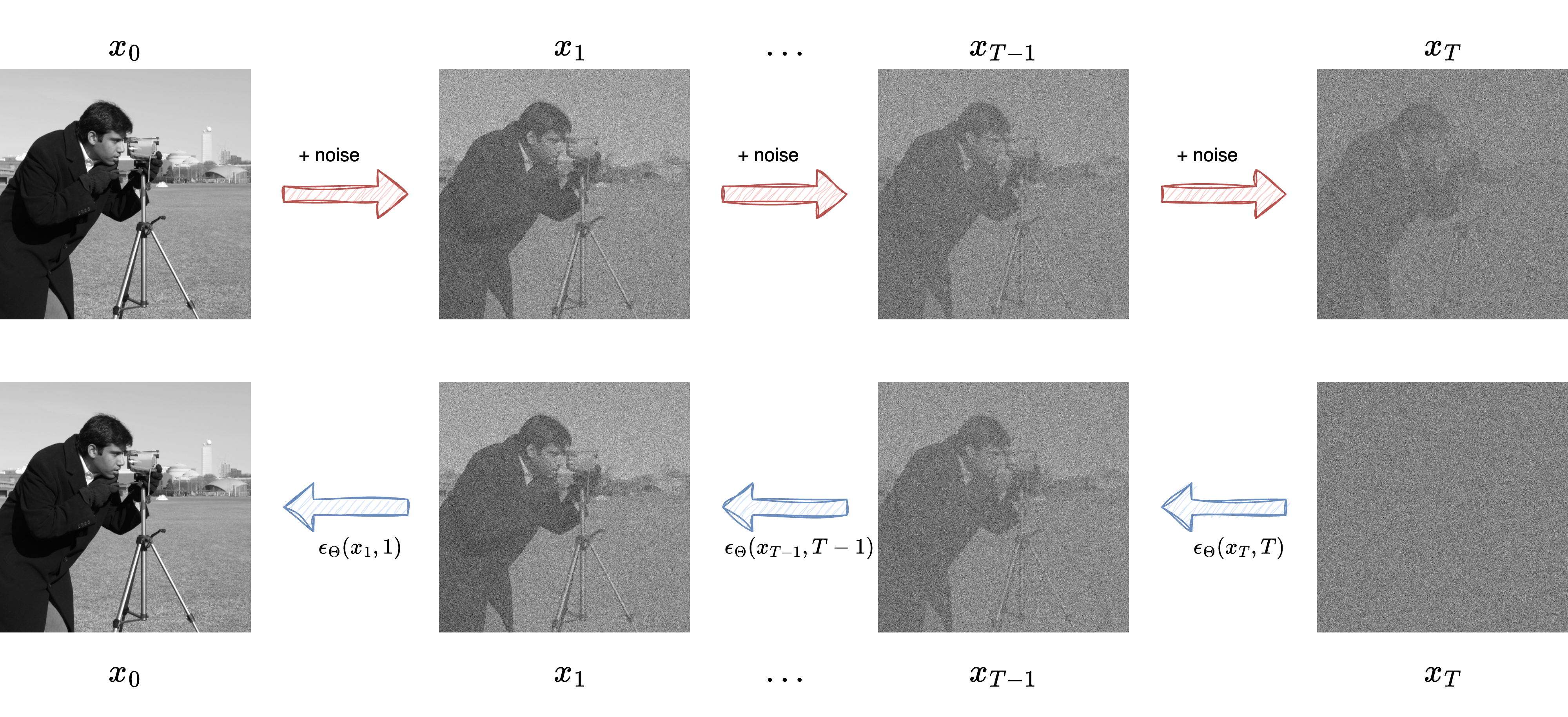
Diffusion models approach generation through a two-step process:
Forward process: gradually adds noise to data over time
Reverse process: learns to remove noise step-by-step
The reverse process is modeled using deep neural networks trained to denoise. This results in a powerful generative model with high sample fidelity.
In the next chapter, we will explore more in detail the working mechanism of Diffusion Models.