Diffusion Models for Image Generation

Diffusion Models for Image Generation#

As previously introduced, in this final chapter we will discuss more in details the working mechanism of Diffusion Models, the state-of-the-art for image generation.

Introduction to Diffusion Models#

Diffusion models are a class of generative models that produce data samples by iteratively denoising a Gaussian noise vector. Unlike GANs or VAEs, they are likelihood-based models that combine principles from non-equilibrium thermodynamics and probabilistic modeling.

The key idea is to define a Markov chain that slowly destroys the structure of data by adding Gaussian noise over several steps, and then train a neural network to reverse this noising process, recovering the original data.

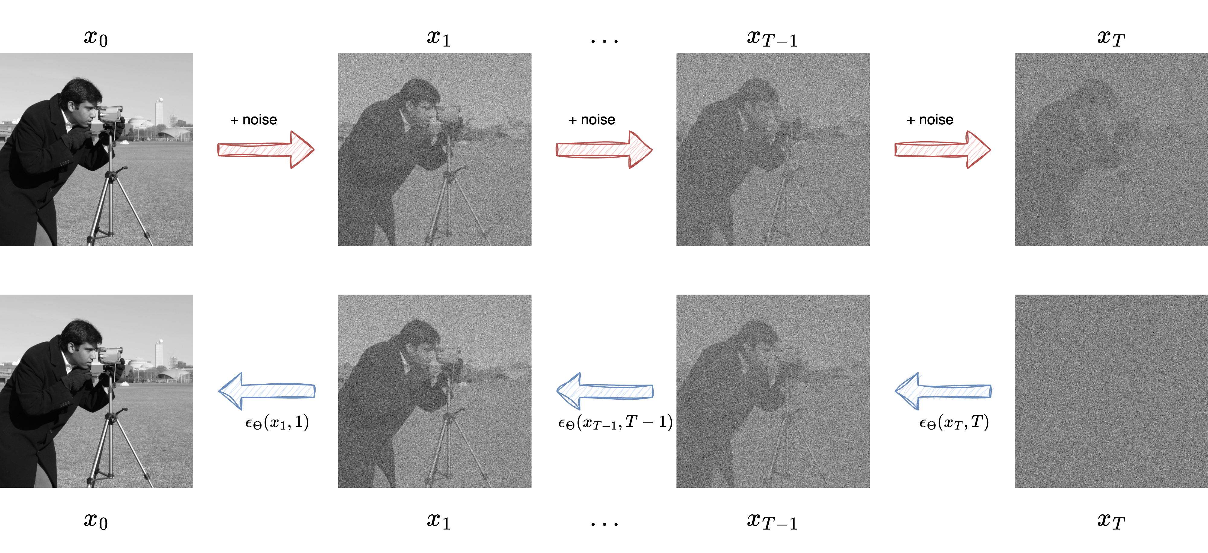
The Forward Process: Gradual Noising#

Let \(x_0 \sim p_{\text{data}}(x)\) be a sample from the real data distribution.

We define a sequence of latent variables \(x_1, x_2, \ldots, x_T\) where noise is added at each step according to a predefined variance schedule \( \beta_1, \dots, \beta_T\). The forward (noising) process is defined as:

\[ q(x_t \mid x_{t-1}) = \mathcal{N}(x_t; \sqrt{1 - \beta_t} \, x_{t-1}, \beta_t I) \]

This is a Markov process that gradually transforms the data into pure noise.

We can also write the marginal distribution of \(x_t\) directly given \(x_0\) as:

\[ q(x_t \mid x_0) = \mathcal{N}(x_t; \sqrt{\bar{\alpha}_t} x_0, (1 - \bar{\alpha}_t) I) \]

where:

\[ \alpha_t = 1 - \beta_t, \quad \bar{\alpha}_t = \prod_{s=1}^t \alpha_s \]

Intuitively, as \(t \to T\), \(x_t\) becomes close to an isotropic Gaussian \(\mathcal{N}(0, I)\).

The Reverse Process: Learning to Denoise#

Our goal is to learn the reverse-time process:

\[ p_\theta(x_{t-1} \mid x_t) \]

Unlike the forward process, this is not known analytically. We approximate it using a neural network parameterized by \(\theta\).

Assuming a Gaussian form for the reverse conditional:

\[ p_\theta(x_{t-1} \mid x_t) = \mathcal{N}(x_{t-1}; \mu_\theta(x_t, t), \Sigma_\theta(x_t, t)) \]

Most models fix \(\Sigma_\theta\) and train the network to predict only the mean (or alternatively the noise that was added, as we’ll see next).

Denoising Score Matching (Simplified View)#

Rather than modeling the full posterior \(p_\theta(x_{t-1} \mid x_t)\), the training objective is simplified by using denoising score matching. The network learns to predict the noise \(\epsilon\) added at each step:

\[ x_t = \sqrt{\bar{\alpha}_t} x_0 + \sqrt{1 - \bar{\alpha}_t} \, \epsilon, \quad \epsilon \sim \mathcal{N}(0, I) \]

A neural network \(\epsilon_\theta(x_t, t)\) is trained to minimize the expected squared error:

\[ \mathcal{L}_{\text{simple}}(\theta) = \mathbb{E}_{x_0, \epsilon, t} \left[ \left\| \epsilon - \epsilon_\theta(x_t, t) \right\|^2 \right] \]

This formulation greatly simplifies training and leads to excellent sample quality.

Summary of Diffusion Model Structure#

Forward process: adds small amounts of Gaussian noise step-by-step to data
Reverse process: learned by a neural network to denoise
Final sample generation: starts from pure Gaussian noise and applies the learned denoising steps

This framework allows for stable training, unlike GANs, and for high-quality image synthesis, often outperforming VAEs and GANs in perceptual quality.

Training Diffusion Models#

Once we have defined the forward noising process and the reverse denoising model, the training phase consists in teaching the neural network to predict the noise that was added to a clean image.

We use a time-dependent neural network \(\epsilon_\theta(x_t, t)\) that receives as input a noisy image \(x_t\) and a timestep \(t\), and tries to estimate the noise \(\epsilon\) used to corrupt the original clean image \(x_0\).

Recap: Sampling from the Forward Process#

Recall that we can sample a noisy image \(x_t\) directly given the clean image \(x_0\) as:

\[ x_t = \sqrt{\bar{\alpha}_t} \, x_0 + \sqrt{1 - \bar{\alpha}_t} \, \epsilon, \quad \epsilon \sim \mathcal{N}(0, I) \]

This gives us a way to synthetically generate training data pairs ((x_t, \epsilon)) from a dataset of real images \(x_0\).

The Loss Function#

The model is trained by minimizing the mean squared error between the predicted noise and the actual sampled noise:

\[ \mathcal{L}_{\text{simple}}(\theta) = \mathbb{E}_{x_0, \epsilon, t} \left[ \left\| \epsilon - \epsilon_\theta(x_t, t) \right\|^2 \right] \]

This approach has the following advantages:

It avoids explicitly computing the reverse conditional distribution.
It is simple to implement.
It works well in practice.

Training Procedure in PyTorch#

Here is a minimal example of how this training step might look like using PyTorch:

import torch
import torch.nn as nn

def get_alphas(beta_schedule):
    beta = torch.tensor(beta_schedule)
    alpha = 1.0 - beta
    alpha_bar = torch.cumprod(alpha, dim=0)
    return alpha, alpha_bar

class SimpleUNet(nn.Module):
    def __init__(self):
        super().__init__()
        # Minimal UNet-like model for illustration
        self.net = nn.Sequential(
            nn.Conv2d(3, 64, 3, padding=1),
            nn.ReLU(),
            nn.Conv2d(64, 64, 3, padding=1),
            nn.ReLU(),
            nn.Conv2d(64, 3, 3, padding=1),
        )

    def forward(self, x, t):
        # Embed time as additional channel or via positional encoding
        return self.net(x)

# Assume we already have: x0: (B, C, H, W), sampled from data
# t: timestep indices uniformly sampled in [1, T]
def sample_xt(x0, t, alpha_bar):
    sqrt_alpha_bar = torch.sqrt(alpha_bar[t])[:, None, None, None]
    sqrt_one_minus_alpha_bar = torch.sqrt(1 - alpha_bar[t])[:, None, None, None]
    noise = torch.randn_like(x0)
    xt = sqrt_alpha_bar * x0 + sqrt_one_minus_alpha_bar * noise
    return xt, noise

# Training step
def training_step(model, x0, t, alpha_bar, optimizer):
    xt, noise = sample_xt(x0, t, alpha_bar)
    pred_noise = model(xt, t)
    loss = nn.MSELoss()(pred_noise, noise)
    optimizer.zero_grad()
    loss.backward()
    optimizer.step()
    return loss.item()

Image Generation#

Once the model has been trained to predict the noise added during the forward process, we can generate new images by reversing the diffusion process. This process begins from pure Gaussian noise and proceeds step-by-step, applying the learned denoising network.

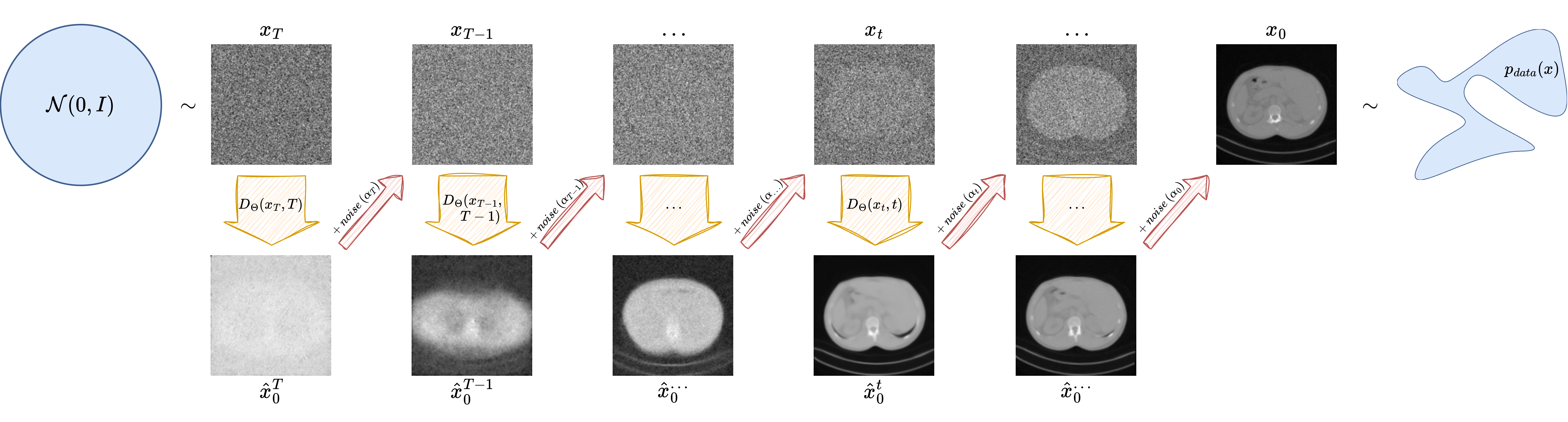
The Reverse Sampling Process#

Given a trained model \(\epsilon_\theta(x_t, t)\), we start from \(x_T \sim \mathcal{N}(0, I)\) and apply the following iterative update:

\[ x_{t-1} = \frac{1}{\sqrt{\alpha_t}} \left( x_t - \frac{1 - \alpha_t}{\sqrt{1 - \bar{\alpha}_t}} \epsilon_\theta(x_t, t) \right) + \sigma_t z \]