Diffusion Models for Inverse Problems#
Once a generative model has been trained, it can be used as a prior for reconstruction. The central idea is probabilistic: instead of searching for an image that only fits the measured datum, we search for an image that is both data-consistent and plausible under the learned image distribution.
This notebook focuses on diffusion models as priors for inverse problems. We start from the Bayesian viewpoint, explain why diffusion models are particularly attractive in this setting, and then discuss two representative methods: DPS [7] and DiffPIR [46]. The emphasis is on the logic of the algorithms and on explicit code. The implementations below are intentionally compact and pedagogical: they are meant to expose the main update ideas, not to reproduce the full engineering details of the original papers. In particular, the code should be read as DPS-style and DiffPIR-style reconstruction rather than as exact research implementations.
Bayesian Viewpoint and Diffusion Priors#
Let the measurement model be
where \(K\) is a known forward operator and \(\boldsymbol{e}\) is the measurement noise. If the noise is Gaussian with variance \(\sigma_y^2\), then the likelihood is
If we also have a prior distribution \(p(\boldsymbol{x})\) for realistic images, the posterior is
This formula says that reconstruction should combine two pieces of information: the likelihood, which measures agreement with the data, and the prior, which measures plausibility of the image.
Latent-variable models such as VAEs and GANs already provide a learned prior, but they constrain the solution to the range of a low-dimensional generator. Diffusion models [18, 37] are richer. Instead of restricting the image to lie on a fixed latent manifold, they learn how to denoise realistic images across many noise levels. This gives access to two closely related objects: a noise predictor \(\boldsymbol{\epsilon}_\Theta(\boldsymbol{x}_t,t)\) and the corresponding clean-image estimate
In posterior-sampling methods, this estimate is repeatedly combined with the measurement model. The result is a family of algorithms that alternate, in different ways, between a diffusion prior step and a data-consistency step.
It is worth being precise about what the prior means here. A diffusion model usually does not give us a tractable closed-form density \(p(\boldsymbol{x})\). What it gives us is denoising information, or equivalently score information for noisy versions of the data distribution. This is enough to guide iterative reconstruction, because the algorithm can repeatedly ask: among images that fit the measurements, in which direction does the learned model regard the image as becoming more realistic?
Note
The code cells below assume that the diffusion model from the previous notebook has already been trained and saved in ../weights/DDPMDenoiser.pth. They also assume the same architecture and preprocessing choices used there.
import glob
import math
import sys
from pathlib import Path

import matplotlib.pyplot as plt
import numpy as np
import torch
from PIL import Image
from torch.utils.data import DataLoader, Dataset
from torchvision import transforms

sys.path.append('..')
from IPPy import operators, utilities
from IPPy.nn.diffusion import DiffusionUNet, cosine_beta_schedule, denormalize_to_01, extract

book_root = Path('..').resolve()
weights_dir = book_root / 'weights'
weights_path = weights_dir / 'DDPMDenoiser.pth'


class MayoDataset(Dataset):
    def __init__(self, data_path, data_shape=64):
        super().__init__()
        self.fname_list = sorted(glob.glob(f'{data_path}/*/*.png'))
        self.transform = transforms.Compose([
            transforms.Resize((data_shape, data_shape), antialias=True),
            transforms.ToTensor(),
            transforms.Normalize((0.5,), (0.5,)),
        ])

    def __len__(self):
        return len(self.fname_list)

    def __getitem__(self, idx):
        x = Image.open(self.fname_list[idx]).convert('L')
        return self.transform(x)


def make_beta_schedule(num_steps):
    return cosine_beta_schedule(num_steps)


def predict_x0_from_eps(x_t, eps_pred, t, alpha_bars):
    return (x_t - extract((1 - alpha_bars).sqrt(), t, x_t.shape) * eps_pred) / extract(alpha_bars.sqrt(), t, x_t.shape)


def deterministic_ddim_update(x_t, x0_hat, eps_pred, t_next, alpha_bars):
    if t_next < 0:
        return x0_hat
    alpha_bar_next = alpha_bars[t_next].to(x_t.device)
    return torch.sqrt(alpha_bar_next) * x0_hat + torch.sqrt(1 - alpha_bar_next) * eps_pred


device = utilities.get_device()
num_diffusion_steps = 400
betas = make_beta_schedule(num_diffusion_steps)
alphas = 1.0 - betas
alpha_bars = torch.cumprod(alphas, dim=0)

test_dataset = MayoDataset(data_path=str(book_root / 'Mayo' / 'test'), data_shape=64)
if not weights_path.exists():
    raise FileNotFoundError(f'Diffusion weights not found at {weights_path}. Train the previous notebook first.')

model = DiffusionUNet(
    in_ch=1,
    base_ch=64,
    channel_mults=(1, 2, 4),
    time_dim=256,
    dropout=0.05,
    attn_levels=(1, 2),
)
model.load_state_dict(torch.load(weights_path, map_location='cpu'))
model = model.to(device)
model.eval()

K = operators.Blurring(
    img_shape=(64, 64),
    kernel_type='motion',
    kernel_size=9,
    motion_angle=20,
)

print('Device:', device)
print('Loaded diffusion weights from:', weights_path)
print('Diffusion steps:', num_diffusion_steps)
Device: cuda
Loaded diffusion weights from: C:\Users\tivog\computational-imaging\years\2025-26\weights\DDPMDenoiser.pth
Diffusion steps: 400
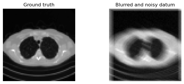
with torch.no_grad():
    x_true = test_dataset[0].unsqueeze(0).to(device)
    y_delta = K(x_true)
    y_delta = y_delta + utilities.gaussian_noise(y_delta, noise_level=0.01)

plt.figure(figsize=(8, 3))
plt.subplot(1, 2, 1)
plt.imshow(denormalize_to_01(x_true).cpu().squeeze(), cmap='gray')
plt.title('Ground truth')
plt.axis('off')

plt.subplot(1, 2, 2)
plt.imshow(denormalize_to_01(y_delta).cpu().squeeze(), cmap='gray')
plt.title('Blurred and noisy datum')
plt.axis('off')

plt.tight_layout()
plt.show()
DPS and DiffPIR#
The two methods discussed below both use the same trained diffusion prior, but they combine it with the measurement model in different ways.
DPS uses a likelihood gradient during the reverse diffusion process.
DiffPIR follows a plug-and-play philosophy and alternates between a denoising step and a data-consistency step.
The graphics below are meant to make this distinction concrete. In each column, we look at one representative reverse-diffusion timestep. The top row shows the current state \(\boldsymbol{x}_t\), the middle row shows the clean-image estimate \(\hat{\boldsymbol{x}}_0(\boldsymbol{x}_t,t)\) produced by the denoiser, and the bottom row shows a data-consistent projection
where \(C(\cdot)\) denotes a correction toward agreement with the measurements. The important conceptual point is that the diffusion model does not directly return the final reconstruction. It returns a prior-driven estimate, and the inverse-problem method decides how that estimate is combined with the physics encoded by \(K\) and the datum \(\boldsymbol{y}^\delta\).
The code that follows is deliberately compact and pedagogical. It captures the main update logic of each method, but it should not be confused with a full research-grade implementation. The purpose is to make the algorithmic philosophy transparent: where does the diffusion prior enter, where does the measurement model enter, and how are the two balanced at each iteration?
DPS: Diffusion Posterior Sampling#
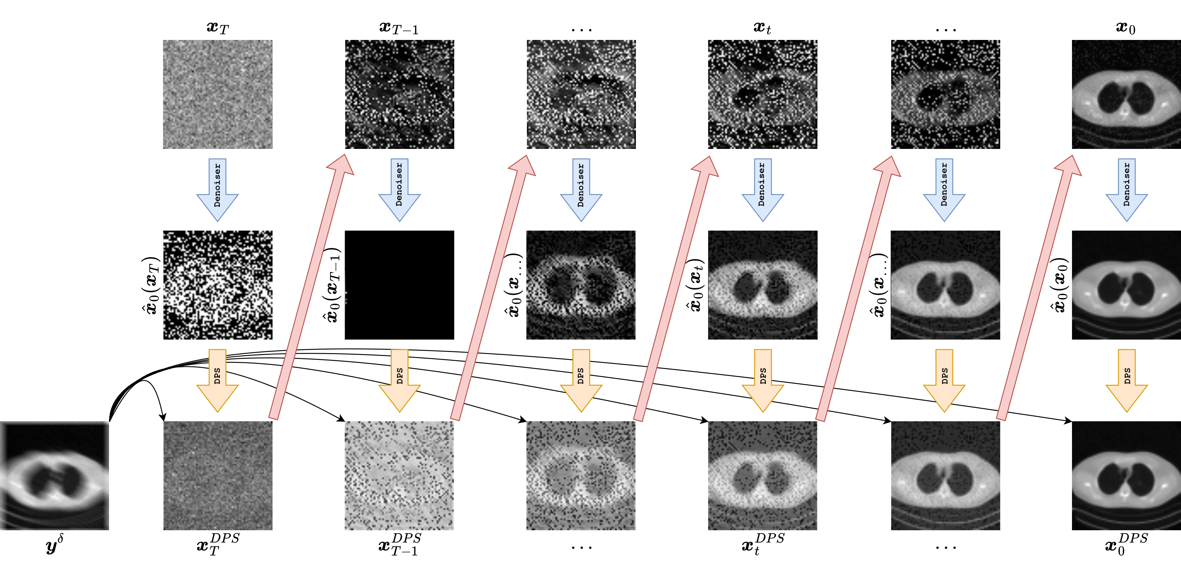
The figure above should be read from top to bottom at each selected timestep. The state \(\boldsymbol{x}_t\) is the current noisy iterate of the reverse process. The denoiser then produces a clean-image estimate \(\hat{\boldsymbol{x}}_0\), and from that estimate one can evaluate how well the reconstruction matches the measurements. DPS uses that mismatch not as a separate projection step, but as a gradient signal that modifies the reverse diffusion trajectory itself.
The starting point is the Bayesian posterior
At diffusion time \(t\), one would ideally like to sample from a time-dependent posterior \(p_t(\boldsymbol{x}_t \mid \boldsymbol{y}^\delta)\). In score-based language, this requires the score
The first term is supplied by the diffusion model, while the second comes from the measurement model. For Gaussian noise, the likelihood term is proportional to
In practice, we do not know how to evaluate this quantity exactly at \(\boldsymbol{x}_t\), because the measurements are naturally compared to a clean image rather than to a noisy latent state. DPS resolves this by using the denoiser-induced estimate \(\hat{\boldsymbol{x}}_0(\boldsymbol{x}_t,t)\) as a proxy for the underlying clean image and then differentiating the data-fidelity term through that estimate. This gives a guidance direction of the form
which is then used to steer the reverse step. In the pedagogical code below, this appears as a DDIM-style update followed by a correction in the direction of negative likelihood gradient. Symbolically, one may think of the update as
where \(R_\Theta\) denotes the prior-driven reverse diffusion step and \(\eta\) is a guidance strength.
This viewpoint has a major advantage: DPS keeps the diffusion prior fully in the loop and adapts it to the inverse problem without retraining the generative model. It is also flexible: as long as one can compute or approximate a likelihood gradient, the same prior can be reused across different forward operators. This makes DPS conceptually attractive for a course on computational imaging, because it separates prior learning from data acquisition.
The limitations are equally important. First, the method is computationally heavy because every reverse step requires both a denoiser evaluation and a gradient-based data-consistency correction. Second, the guidance strength must be tuned carefully: if it is too small, the reconstruction can ignore the measurements and drift toward visually plausible but data-inconsistent images; if it is too large, the sampler can become unstable or oversharpened. Third, the likelihood gradient is only approximate, because it is routed through \(\hat{\boldsymbol{x}}_0\) rather than through an exact posterior model. So DPS should be understood as a practically effective posterior-guided sampler, not as a black-box guarantee of exact Bayesian sampling.
In the simplified code below, the key idea is preserved by computing a likelihood-based correction from the current clean-image estimate and using it to steer the next iterate. The bottom row of the graphic is therefore not the actual DPS state update itself, but an interpretable visualization of the data-consistency direction suggested by the measurements.
def dps_reconstruct(model, y_delta, K, alpha_bars, sigma_y=0.01, sample_steps=40, guidance_scale=0.15):
    schedule = torch.linspace(num_diffusion_steps - 1, 0, sample_steps, dtype=torch.long, device=device)
    x = torch.randn_like(y_delta)

    for i in range(len(schedule) - 1):
        t_current = int(schedule[i].item())
        t_next = int(schedule[i + 1].item())
        t = torch.full((x.shape[0],), t_current, device=device, dtype=torch.long)

        x = x.detach().requires_grad_(True)
        eps_pred = model(x, t)
        x0_hat = predict_x0_from_eps(x, eps_pred, t, alpha_bars).clamp(-1.0, 1.0)
        data_loss = torch.mean((K(x0_hat) - y_delta) ** 2) / (2 * sigma_y ** 2)
        grad = torch.autograd.grad(data_loss, x)[0]

        with torch.no_grad():
            x_next = deterministic_ddim_update(x, x0_hat, eps_pred, t_next, alpha_bars)
            x = (x_next - guidance_scale * grad).clamp(-1.0, 1.0)

    with torch.no_grad():
        t0 = torch.zeros((x.shape[0],), device=device, dtype=torch.long)
        eps_pred = model(x, t0)
        return predict_x0_from_eps(x, eps_pred, t0, alpha_bars).clamp(-1.0, 1.0).detach()


x_dps = dps_reconstruct(model, y_delta, K, alpha_bars, sigma_y=0.01, sample_steps=40, guidance_scale=0.15)
DiffPIR: Diffusion Plug-and-Play Image Restoration#
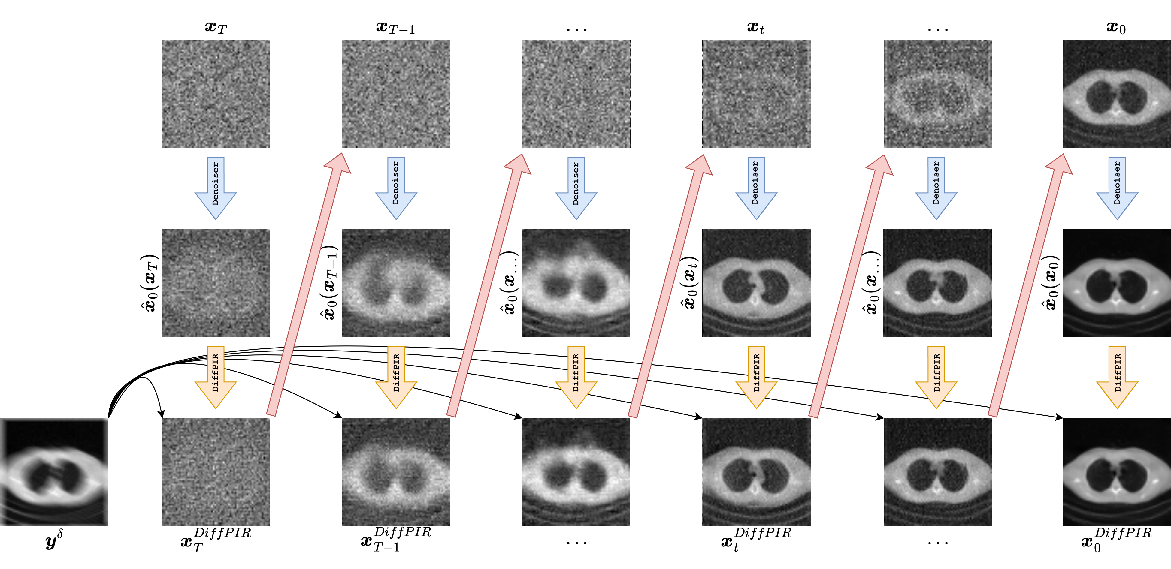
The DiffPIR graphic is easier to read as an operator-splitting picture. At each timestep, we start from a current state \(\boldsymbol{x}_t\), use the diffusion model to produce a prior-driven estimate \(\hat{\boldsymbol{x}}_0\), and then explicitly apply a data-consistency map
before moving to the next iterate. In other words, prior information and measurement consistency are handled in two conceptually distinct substeps.
DiffPIR follows a plug-and-play philosophy. Instead of trying to write down one exact posterior transition, it alternates between two operations: a diffusion-model denoising step, which pushes the iterate toward the learned image prior, and a data-consistency step, which pushes it back toward agreement with the measurements. This is conceptually close to classical plug-and-play and proximal algorithms, except that the denoiser is now replaced by a diffusion prior.
Mathematically, the philosophy is the following. Suppose one wants to minimize an objective that balances data fidelity and regularization,
In classical plug-and-play methods, one replaces the explicit regularizer \(\mathcal{R}\) by a denoiser or a proximal-like map. DiffPIR does something analogous with a diffusion model: it treats the denoising action of the reverse process as an implicit learned prior and combines it with a correction driven by the forward operator. In the pedagogical code below, the prior part is implemented by a deterministic DDIM-style step producing a denoised candidate \(\boldsymbol{x}_{\mathrm{prior}}\), and the data-consistency part is a correction of the form
where \(\tau > 0\) plays the role of a step size. This is nothing but a gradient-descent correction for the quadratic data-fidelity term. The denoiser and the forward model therefore act in alternation: the denoiser improves plausibility, and the explicit correction restores physical consistency.
This point of view is very useful pedagogically because it connects diffusion methods to a much older inverse-problems tradition. It is also practically attractive. DiffPIR is modular, relatively easy to interpret, and often more stable to tune than posterior-guided samplers, because the roles of the two substeps are clearly separated. When one looks at the graphic, the bottom row really is the heart of the method: after each prior step, the algorithm visibly projects the estimate back toward the measurement model.
Its advantages are therefore modularity, interpretability, and conceptual closeness to optimization. One can often adapt the data-consistency step to the structure of the operator \(K\) quite naturally, and one can reason about the parameter \(\tau\) as a standard optimization step size. DiffPIR also tends to produce reconstructions that remain visibly tethered to the measurements, because data consistency is imposed explicitly at every iteration.
The limitations come from the same splitting structure. The method is not derived here as an exact posterior sampler, so one should not automatically interpret its iterates as samples from the true Bayesian posterior. Its behavior depends strongly on the balance between denoising and correction: if the denoising step is too dominant, the result can hallucinate plausible but incorrect detail; if the data-consistency step is too strong, the method can become oversmoothed or oscillatory. Moreover, the clean separation between prior and data terms is algorithmically convenient, but it may be less faithful to the true posterior geometry than methods that couple both ingredients more tightly.
So, in short, DPS is closer to the idea of steering a posterior diffusion trajectory, whereas DiffPIR is closer to alternating a learned denoiser with an optimization-style correction. The code below intentionally emphasizes this difference.
def diffpir_reconstruct(model, y_delta, K, alpha_bars, sample_steps=40, tau=0.6):
    schedule = torch.linspace(num_diffusion_steps - 1, 0, sample_steps, dtype=torch.long, device=device)
    x = y_delta.clone()

    for i in range(len(schedule) - 1):
        t_current = int(schedule[i].item())
        t_next = int(schedule[i + 1].item())
        t = torch.full((x.shape[0],), t_current, device=device, dtype=torch.long)

        with torch.no_grad():
            eps_pred = model(x, t)
            x0_hat = predict_x0_from_eps(x, eps_pred, t, alpha_bars).clamp(-1.0, 1.0)
            x_prior = deterministic_ddim_update(x, x0_hat, eps_pred, t_next, alpha_bars)
            residual = K(x_prior) - y_delta
            x = (x_prior - tau * K.T(residual)).clamp(-1.0, 1.0)

    return x.clamp(-1.0, 1.0).detach()


x_diffpir = diffpir_reconstruct(model, y_delta, K, alpha_bars, sample_steps=40, tau=0.6)
Comparing the Reconstructions#
The cell below compares the reconstructions obtained with the three methods on the same blurred measurement. The quantitative numbers are only indicative, because the implementations here are deliberately simplified for teaching. The important point is to see that one and the same diffusion prior can be combined with the measurement model in multiple algorithmic ways.
A good way to read the comparison is not to ask only which image looks best, but also which algorithm seems to emphasize likelihood guidance, explicit operator structure, or plug-and-play balancing most strongly.
def mse(x, y):
    x_01 = denormalize_to_01(x.detach())
    y_01 = denormalize_to_01(y.detach())
    return torch.mean((x_01 - y_01) ** 2).item()


def psnr(x, y):
    mse_val = mse(x, y)
    return float('inf') if mse_val == 0 else -10 * math.log10(mse_val)


def ssim(x, y, window_size=11, sigma=1.5, c1=0.01 ** 2, c2=0.03 ** 2):
    x_01 = denormalize_to_01(x.detach())
    y_01 = denormalize_to_01(y.detach())
    coords = torch.arange(window_size, device=x_01.device, dtype=x_01.dtype) - window_size // 2
    gauss = torch.exp(-(coords ** 2) / (2 * sigma ** 2))
    gauss = gauss / gauss.sum()
    window_2d = torch.outer(gauss, gauss)
    window = window_2d.expand(x_01.shape[1], 1, window_size, window_size).contiguous()
    mu_x = torch.nn.functional.conv2d(x_01, window, padding=window_size // 2, groups=x_01.shape[1])
    mu_y = torch.nn.functional.conv2d(y_01, window, padding=window_size // 2, groups=y_01.shape[1])
    mu_x2 = mu_x ** 2
    mu_y2 = mu_y ** 2
    mu_xy = mu_x * mu_y
    sigma_x2 = torch.nn.functional.conv2d(x_01 * x_01, window, padding=window_size // 2, groups=x_01.shape[1]) - mu_x2
    sigma_y2 = torch.nn.functional.conv2d(y_01 * y_01, window, padding=window_size // 2, groups=y_01.shape[1]) - mu_y2
    sigma_xy = torch.nn.functional.conv2d(x_01 * y_01, window, padding=window_size // 2, groups=x_01.shape[1]) - mu_xy
    ssim_map = ((2 * mu_xy + c1) * (2 * sigma_xy + c2)) / ((mu_x2 + mu_y2 + c1) * (sigma_x2 + sigma_y2 + c2))
    return ssim_map.mean().item()


results = {
    'Observation': y_delta,
    'DPS': x_dps,
    'DiffPIR-style': x_diffpir,
}

fig, axes = plt.subplots(1, 4, figsize=(12, 3))
axes[0].imshow(denormalize_to_01(x_true.detach()).cpu().squeeze(), cmap='gray')
axes[0].set_title('Ground truth')
axes[0].axis('off')

for ax, (name, image) in zip(axes[1:], results.items()):
    ax.imshow(denormalize_to_01(image.detach()).cpu().squeeze(), cmap='gray')
    if name == 'Observation':
        ax.set_title(name)
    else:
        ax.set_title(f'{name}\nPSNR: {psnr(image, x_true):.2f} dB\nSSIM: {ssim(image, x_true):.3f}')
    ax.axis('off')

plt.tight_layout()
plt.show()

for name, image in results.items():
    print(f'{name:>14} | MSE: {mse(image, x_true):.6f} | PSNR: {psnr(image, x_true):.3f} dB | SSIM: {ssim(image, x_true):.4f}')
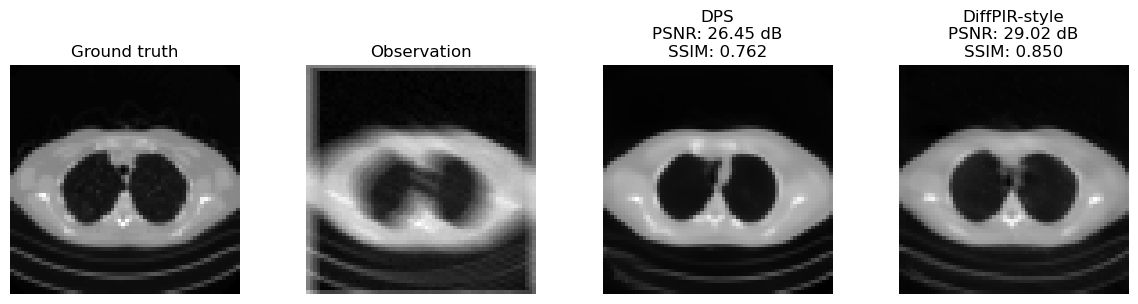
   Observation | MSE: 0.006219 | PSNR: 22.063 dB | SSIM: 0.6291
           DPS | MSE: 0.002263 | PSNR: 26.454 dB | SSIM: 0.7623
 DiffPIR-style | MSE: 0.001253 | PSNR: 29.022 dB | SSIM: 0.8502
Limitations and Points of Attention#
Diffusion-based reconstruction methods are powerful, but they require careful interpretation.
They are computationally expensive, because each reconstruction requires many neural-network evaluations.
They are sensitive to the forward model. If the operator \(K\) used at test time is mismatched, the method may deteriorate badly.
They can produce visually convincing images that are not fully data-consistent if the likelihood term is too weak or badly tuned.
Hyperparameters such as the guidance strength, the noise schedule, and the number of sampling steps strongly affect the result.
A posterior sampler should, in principle, represent uncertainty. In practice, many simplified implementations collapse toward a single preferred solution.
Posterior plausibility is not the same thing as ground-truth correctness: if the measurements are weak or the learned image model is biased, the algorithm may return a highly realistic but wrong image.
Distribution shift remains a serious issue. A diffusion prior trained on one image population may behave poorly on anatomies, textures, or acquisition settings that were absent from training.
It is also worth noting that the ecosystem is broader than the two methods discussed here. Related approaches include DDNM for noiseless linear inverse problems and many other variants that combine diffusion priors with optimization, proximal methods, or plug-and-play schemes.
Warning
A diffusion-based reconstruction can look extremely convincing even when it is not the correct posterior sample, or even when it is not fully consistent with the measured data. This is why quantitative evaluation and careful inspection of data consistency remain essential.
Exercises#
In the Bayesian formulation, what are the respective roles of the likelihood and the prior?
Why can a diffusion model be interpreted as a learned image prior?
What is the main algorithmic idea behind DPS?
What is the plug-and-play philosophy behind DiffPIR?
Code exercise: change the blur angle or kernel size and compare how the two methods react.
Code exercise: vary the DPS guidance scale or the DiffPIR parameter
tauand observe the effect on reconstruction quality.Code exercise: generate two different DPS reconstructions from different random initializations and compare them. What does this say about posterior sampling?
Further Reading#
For the Bayesian and inverse-problem background, see [21] and [3]. For diffusion posterior sampling, see [7]. For DiffPIR, see [46]. For a related method in the noiseless linear setting, see [41].