Deep dive into IPPy#
In this notebook we move from plain PyTorch to IPPy, with a concrete inverse-problem example based on motion deblurring. The goal is not to introduce all the theory at once, but to show a complete workflow:
load Mayo slices with the same custom
Datasetused in the previous section;build a synthetic forward model with an
IPPyoperator;generate blurred and noisy measurements;
train a small convolutional neural network to recover the clean image;
evaluate the reconstruction quality with
PSNRandSSIMfromIPPy.
IPPy is a small library developed for this course to simplify inverse problems and image reconstruction experiments. It includes:
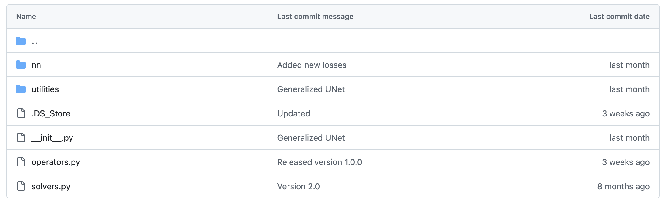
operators: forward models such as blurring, downscaling, gradients, and CT projectors;solvers: classical reconstruction algorithms, useful as references and baselines;nn: neural-network architectures and training utilities;utilities: helper functions for metrics, noise generation, visualization, and device handling.
The code for IPPy can be downloaded from: devangelista2/IPPy.
Introduction and requirements#
IPPy is built on top of standard Python tools for tensors, visualization, inverse problems, and image processing. In practice, you will typically need:
torchnumpynumbascikit-imagePILmatplotlibastra-toolboxfor CT experiments
For the motion-deblurring example of this notebook, PyTorch is the main requirement. A GPU is recommended for training, but the example also works on CPU if needed.
Standard tensors#
Most IPPy routines are designed for standardized PyTorch tensors, namely tensors that:
have shape
(N, c, n_x, n_y);are stored as
float32;are normalized in the range
[0, 1].
This is exactly the convention we already adopted in the previous section when preparing images for neural networks.
The operators module#
The core idea of IPPy is simple: an inverse problem starts from a forward operator
where x is the clean image and y is the measured or corrupted datum. In IPPy, these forward models are implemented as Python classes.
The basic Operator interface is:
import sys

sys.path.append("..")

import torch
from IPPy.operators import OperatorFunction


class Operator:
    def __call__(self, x: torch.Tensor) -> torch.Tensor:
        # Applies operator using PyTorch autograd wrapper.
        return OperatorFunction.apply(self, x)

    def __matmul__(self, x: torch.Tensor) -> torch.Tensor:
        # Matrix-vector multiplication.
        return self.__call__(x)

    def T(self, y: torch.Tensor) -> torch.Tensor:
        # Transpose operator (adjoint).
        device = y.device
        return self._adjoint(y).to(device).requires_grad_(True)

    def _matvec(self, x: torch.Tensor) -> torch.Tensor:
        # Apply the operator to a single `(c, h, w)` tensor.
        raise NotImplementedError

    def _adjoint(self, y: torch.Tensor) -> torch.Tensor:
        # Apply the adjoint operator to a single `(c, h, w)` tensor.
        raise NotImplementedError
The important point is that the user only needs to define:
_matvec, the forward actionK(x);_adjoint, the adjoint actionK^T(y).
Everything else is handled so that the operator works naturally with PyTorch tensors and backpropagation.
A first toy example#
Before moving to motion blur, let us define a very simple operator: the image negative. This is not a meaningful inverse problem, but it is a good first example because we can immediately see what the operator does.
In the next code cell we also reuse the same MayoDataset implementation from the previous section.
# -----------------
# This is just for rendering on the website
import sys

sys.path.append("..")
# -----------------

import glob

import matplotlib.pyplot as plt
import numpy as np
import torch.nn.functional as F
from PIL import Image
from torch.utils.data import Dataset

from IPPy import metrics, operators, solvers, utilities


class NegativeOperator(operators.Operator):
    def _matvec(self, x):
        # Since x is normalized in [0, 1], its negative is just 1 - x.
        return 1 - x

    def _adjoint(self, y):
        # For this toy operator, the adjoint has the same expression.
        return 1 - y


class MayoDataset(Dataset):
    def __init__(self, data_path, data_shape):
        super().__init__()

        self.data_path = data_path
        self.data_shape = data_shape

        # We expect data_path to be like "./data/Mayo/train" or "./data/Mayo/test"
        self.fname_list = glob.glob(f"{data_path}/*/*.png")

    def __len__(self):
        return len(self.fname_list)

    def __getitem__(self, idx):
        # Load the idx's image from fname_list
        img_path = self.fname_list[idx]

        # To load the image as grey-scale
        x = Image.open(img_path).convert("L")

        # Convert to numpy array -> (512, 512)
        x = np.array(x)

        # Convert to pytorch tensor -> (1, 512, 512) <-> (c, n_x, n_y)
        x = torch.tensor(x).unsqueeze(0)

        # Resize to the required shape
        x = F.interpolate(
            x.unsqueeze(0).float(),
            size=(self.data_shape, self.data_shape),
            mode="bilinear",
            align_corners=False,
        ).squeeze(0)

        # Normalize in [0, 1] range
        x = (x - x.min()) / (x.max() - x.min())

        return x

    def get_patient_and_slice(self, idx):
        '''
        A utility function. Given an idx, it returns the patient ID and the number of slice of
        that patient corresponding to the idx's datapoint.
        '''
        fname = self.fname_list[idx]
        patient_id = fname.split("/")[-2]
        slice_n = fname.split("/")[-1]
        return patient_id, slice_n


test_data = MayoDataset(data_path="../data/Mayo/test", data_shape=256)
x = test_data[0].unsqueeze(0)

K_negative = NegativeOperator()
y_negative = K_negative(x)

plt.figure(figsize=(10, 5))
plt.subplot(1, 2, 1)
plt.imshow(x.squeeze(), cmap="gray")
plt.axis("off")
plt.title("Original")

plt.subplot(1, 2, 2)
plt.imshow(y_negative.squeeze(), cmap="gray")
plt.axis("off")
plt.title("Negative")
plt.show()
---------------------------------------------------------------------------
IndexError                                Traceback (most recent call last)
Cell In[2], line 80
     76         return patient_id, slice_n
     79 test_data = MayoDataset(data_path="../data/Mayo/test", data_shape=256)
---> 80 x = test_data[0].unsqueeze(0)
     82 K_negative = NegativeOperator()
     83 y_negative = K_negative(x)

Cell In[2], line 44, in MayoDataset.__getitem__(self, idx)
     42 def __getitem__(self, idx):
     43     # Load the idx's image from fname_list
---> 44     img_path = self.fname_list[idx]
     46     # To load the image as grey-scale
     47     x = Image.open(img_path).convert("L")

IndexError: list index out of range
Built-in operators#
The toy example above was useful to understand the interface, but in practice we usually work with operators that simulate a real acquisition or degradation process.
IPPy already contains several ready-to-use operators, including:
computed tomography projectors;
blurring operators;
downscaling operators;
gradient operators.
For this notebook we focus on the motion blur case. The forward model is:
where:
xis the clean Mayo slice;Kis a motion-blur operator;eis a small noise term;y^\deltais the measured image available to the network.
This is the main advantage of IPPy: once the dataset is in standard tensor format, building a synthetic inverse problem only requires a few lines of code.
from IPPy import operators, utilities


def synthesize_measurement(x, operator, noise_level=0.01):
    y = operator(x)
    e = utilities.gaussian_noise(y, noise_level=noise_level)
    y_delta = torch.clamp(y + e, 0.0, 1.0)
    return y, y_delta


x_true = test_data[10].unsqueeze(0)

K = operators.Blurring(
    img_shape=(256, 256),
    kernel_type="motion",
    kernel_size=11,
    motion_angle=25,
)

y, y_delta = synthesize_measurement(x_true, K, noise_level=0.01)
x_adj = K.T(y_delta)

plt.figure(figsize=(16, 4))

plt.subplot(1, 4, 1)
plt.imshow(x_true.squeeze(), cmap="gray")
plt.axis("off")
plt.title("Original")

plt.subplot(1, 4, 2)
plt.imshow(K.kernel.squeeze().cpu(), cmap="magma")
plt.axis("off")
plt.title("Motion kernel")

plt.subplot(1, 4, 3)
plt.imshow(y_delta.squeeze(), cmap="gray")
plt.axis("off")
plt.title("Blurred + noise")

plt.subplot(1, 4, 4)
plt.imshow(x_adj.detach().squeeze(), cmap="gray")
plt.axis("off")
plt.title(r"$K^T(y^\delta)$")

plt.show()

print(f"Blurred image PSNR: {metrics.PSNR(y_delta, x_true):0.2f} dB")
print(f"Blurred image SSIM: {metrics.SSIM(y_delta, x_true):0.4f}")
---------------------------------------------------------------------------
IndexError                                Traceback (most recent call last)
Cell In[3], line 11
      7     y_delta = torch.clamp(y + e, 0.0, 1.0)
      8     return y, y_delta
---> 11 x_true = test_data[10].unsqueeze(0)
     13 K = operators.Blurring(
     14     img_shape=(256, 256),
     15     kernel_type="motion",
     16     kernel_size=11,
     17     motion_angle=25,
     18 )
     20 y, y_delta = synthesize_measurement(x_true, K, noise_level=0.01)

Cell In[2], line 44, in MayoDataset.__getitem__(self, idx)
     42 def __getitem__(self, idx):
     43     # Load the idx's image from fname_list
---> 44     img_path = self.fname_list[idx]
     46     # To load the image as grey-scale
     47     x = Image.open(img_path).convert("L")

IndexError: list index out of range
The cell above already contains the full synthetic pipeline:
take a clean image
x_truefrom the dataset;apply the operator
K;add a controlled amount of noise;
obtain the corrupted measurement
y_delta.
This is exactly what we need when preparing supervised training pairs for a reconstruction network.
Backpropagating through IPPy operators#
Another useful feature is that IPPy operators are compatible with PyTorch automatic differentiation. This is important because many modern methods need to differentiate through the forward model.
For example, if
then PyTorch can automatically compute the gradient of f with respect to x.
x_var = test_data[10].unsqueeze(0).clone().requires_grad_(True)

with torch.no_grad():
    _, y_delta = synthesize_measurement(x_var.detach(), K, noise_level=0.005)

f = torch.sum((K(x_var) - y_delta) ** 2)
f.backward()

print(f"Objective value: {f.item():0.4f}")
print(f"Gradient norm: {torch.norm(x_var.grad).item():0.4f}")
---------------------------------------------------------------------------
IndexError                                Traceback (most recent call last)
Cell In[4], line 1
----> 1 x_var = test_data[10].unsqueeze(0).clone().requires_grad_(True)
      3 with torch.no_grad():
      4     _, y_delta = synthesize_measurement(x_var.detach(), K, noise_level=0.005)

Cell In[2], line 44, in MayoDataset.__getitem__(self, idx)
     42 def __getitem__(self, idx):
     43     # Load the idx's image from fname_list
---> 44     img_path = self.fname_list[idx]
     46     # To load the image as grey-scale
     47     x = Image.open(img_path).convert("L")

IndexError: list index out of range
This observation is conceptually important: IPPy is not only a library for generating data, but also a bridge between the forward model and the learning pipeline.
The solvers module#
Before training a neural network, it is worth remembering that IPPy also includes classical reconstruction methods. In this course they are useful as reference baselines: they give us a first reconstruction without introducing trainable parameters.
We only show one example here, because the main goal of this notebook is the learning-based approach.
solver = solvers.ChambollePockTpVUnconstrained(K)

x_rec, _ = solver(
    y_delta,
    lmbda=0.01,
    x_true=x_true,
    starting_point=torch.zeros_like(x_true),
    verbose=False,
)

print(f"Classical reconstruction PSNR: {metrics.PSNR(x_rec, x_true):0.2f} dB")
print(f"Classical reconstruction SSIM: {metrics.SSIM(x_rec, x_true):0.4f}")

plt.figure(figsize=(15, 5))
plt.subplot(1, 3, 1)
plt.imshow(x_true.detach().squeeze(), cmap="gray")
plt.axis("off")
plt.title("Original")

plt.subplot(1, 3, 2)
plt.imshow(y_delta.detach().squeeze(), cmap="gray")
plt.axis("off")
plt.title("Blurred + noise")

plt.subplot(1, 3, 3)
plt.imshow(x_rec.detach().squeeze(), cmap="gray")
plt.axis("off")
plt.title("Classical reconstruction")
plt.show()
---------------------------------------------------------------------------
NameError                                 Traceback (most recent call last)
Cell In[5], line 1
----> 1 solver = solvers.ChambollePockTpVUnconstrained(K)
      3 x_rec, _ = solver(
      4     y_delta,
      5     lmbda=0.01,
   (...)      8     verbose=False,
      9 )
     11 print(f"Classical reconstruction PSNR: {metrics.PSNR(x_rec, x_true):0.2f} dB")

NameError: name 'K' is not defined
From PyTorch to IPPy: training a simple CNN#
We now build the learning part of the pipeline. The key message is:
PyTorch gives us the usual tools for models, losses, optimizers, and dataloaders;
IPPygives us the forward operator, the synthetic measurements, and the reconstruction metrics.
Since the theory of CNNs will be developed in the next section, we keep the architecture intentionally simple. We only need a small model that takes a blurred image as input and outputs a cleaned version of it.
Step 1: prepare training and test data#
We reuse the same MayoDataset as before and create the dataloaders. During training, the clean image x comes from the dataset, while the corrupted datum y_delta is generated online with the motion-blur operator.
from torch.utils.data import DataLoader


device = utilities.get_device()
print(f"Using device: {device}")

train_data = MayoDataset(data_path="../data/Mayo/train", data_shape=256)
test_data = MayoDataset(data_path="../data/Mayo/test", data_shape=256)

train_loader = DataLoader(train_data, batch_size=8, shuffle=True)
test_loader = DataLoader(test_data, batch_size=8, shuffle=False)
Using device: cpu
---------------------------------------------------------------------------
ValueError                                Traceback (most recent call last)
Cell In[6], line 10
      7 train_data = MayoDataset(data_path="../data/Mayo/train", data_shape=256)
      8 test_data = MayoDataset(data_path="../data/Mayo/test", data_shape=256)
---> 10 train_loader = DataLoader(train_data, batch_size=8, shuffle=True)
     11 test_loader = DataLoader(test_data, batch_size=8, shuffle=False)

File /opt/hostedtoolcache/Python/3.11.15/x64/lib/python3.11/site-packages/torch/utils/data/dataloader.py:394, in DataLoader.__init__(self, dataset, batch_size, shuffle, sampler, batch_sampler, num_workers, collate_fn, pin_memory, drop_last, timeout, worker_init_fn, multiprocessing_context, generator, prefetch_factor, persistent_workers, pin_memory_device, in_order)
    392 else:  # map-style
    393     if shuffle:
--> 394         sampler = RandomSampler(dataset, generator=generator)  # type: ignore[arg-type]
    395     else:
    396         sampler = SequentialSampler(dataset)  # type: ignore[arg-type]

File /opt/hostedtoolcache/Python/3.11.15/x64/lib/python3.11/site-packages/torch/utils/data/sampler.py:149, in RandomSampler.__init__(self, data_source, replacement, num_samples, generator)
    144     raise TypeError(
    145         f"replacement should be a boolean value, but got replacement={self.replacement}"
    146     )
    148 if not isinstance(self.num_samples, int) or self.num_samples <= 0:
--> 149     raise ValueError(
    150         f"num_samples should be a positive integer value, but got num_samples={self.num_samples}"
    151     )

ValueError: num_samples should be a positive integer value, but got num_samples=0
Step 2: define a small CNN#
The following model is a minimal convolutional network:
it reads a single-channel image;
it applies a few convolutional filters with ReLU activations;
it outputs another single-channel image in
[0, 1].
This is enough for a first deblurring experiment. Later in the course we will discuss why deeper architectures such as UNet often work better.
from torch import nn


class SimpleDeblurCNN(nn.Module):
    def __init__(self):
        super().__init__()
        self.net = nn.Sequential(
            nn.Conv2d(1, 16, kernel_size=3, padding=1),
            nn.ReLU(),
            nn.Conv2d(16, 32, kernel_size=3, padding=1),
            nn.ReLU(),
            nn.Conv2d(32, 16, kernel_size=3, padding=1),
            nn.ReLU(),
            nn.Conv2d(16, 1, kernel_size=3, padding=1),
            nn.Sigmoid(),
        )

    def forward(self, x):
        return self.net(x)


model = SimpleDeblurCNN().to(device)
model
SimpleDeblurCNN(
  (net): Sequential(
    (0): Conv2d(1, 16, kernel_size=(3, 3), stride=(1, 1), padding=(1, 1))
    (1): ReLU()
    (2): Conv2d(16, 32, kernel_size=(3, 3), stride=(1, 1), padding=(1, 1))
    (3): ReLU()
    (4): Conv2d(32, 16, kernel_size=(3, 3), stride=(1, 1), padding=(1, 1))
    (5): ReLU()
    (6): Conv2d(16, 1, kernel_size=(3, 3), stride=(1, 1), padding=(1, 1))
    (7): Sigmoid()
  )
)
Step 3: train the network#
We optimize the model with a standard mean-squared-error loss:
At the same time, after each epoch, we monitor two image-quality measures from IPPy:
PSNR, which is sensitive to pixel-wise fidelity;SSIM, which is more sensitive to structural similarity.
This is a good habit: a low training loss is useful, but in imaging we also want interpretable reconstruction metrics.
from torch import optim


def evaluate_model(model, data_loader, operator, loss_fn, device, noise_level=0.01):
    model.eval()

    total_loss = 0.0
    total_psnr = 0.0
    total_ssim = 0.0

    with torch.no_grad():
        for x in data_loader:
            x = x.to(device)
            _, y_delta = synthesize_measurement(x, operator, noise_level=noise_level)

            x_pred = torch.clamp(model(y_delta), 0.0, 1.0)

            total_loss += loss_fn(x_pred, x).item()
            total_psnr += metrics.PSNR(x_pred.cpu(), x.cpu())
            total_ssim += metrics.SSIM(x_pred.cpu(), x.cpu())

    n_batches = len(data_loader)
    return {
        "loss": total_loss / n_batches,
        "psnr": total_psnr / n_batches,
        "ssim": total_ssim / n_batches,
    }


loss_fn = nn.MSELoss()
optimizer = optim.Adam(model.parameters(), lr=1e-3)
n_epochs = 3
noise_level = 0.01

history = {
    "train_loss": [],
    "train_psnr": [],
    "train_ssim": [],
    "test_loss": [],
    "test_psnr": [],
    "test_ssim": [],
}

for epoch in range(n_epochs):
    model.train()

    running_loss = 0.0
    running_psnr = 0.0
    running_ssim = 0.0

    for step, x in enumerate(train_loader):
        x = x.to(device)
        _, y_delta = synthesize_measurement(x, K, noise_level=noise_level)

        optimizer.zero_grad()
        x_pred = torch.clamp(model(y_delta), 0.0, 1.0)
        loss = loss_fn(x_pred, x)
        loss.backward()
        optimizer.step()

        running_loss += loss.item()
        running_psnr += metrics.PSNR(x_pred.detach().cpu(), x.detach().cpu())
        running_ssim += metrics.SSIM(x_pred.detach().cpu(), x.detach().cpu())

    n_train_batches = len(train_loader)
    train_loss = running_loss / n_train_batches
    train_psnr = running_psnr / n_train_batches
    train_ssim = running_ssim / n_train_batches

    test_metrics = evaluate_model(
        model,
        test_loader,
        K,
        loss_fn=loss_fn,
        device=device,
        noise_level=noise_level,
    )

    history["train_loss"].append(train_loss)
    history["train_psnr"].append(train_psnr)
    history["train_ssim"].append(train_ssim)
    history["test_loss"].append(test_metrics["loss"])
    history["test_psnr"].append(test_metrics["psnr"])
    history["test_ssim"].append(test_metrics["ssim"])

    print(
        f"Epoch {epoch + 1}/{n_epochs} | "
        f"train loss = {train_loss:0.4f}, train PSNR = {train_psnr:0.2f} dB, train SSIM = {train_ssim:0.4f} | "
        f"test PSNR = {test_metrics['psnr']:0.2f} dB, test SSIM = {test_metrics['ssim']:0.4f}"
    )
---------------------------------------------------------------------------
NameError                                 Traceback (most recent call last)
Cell In[8], line 51
     48 running_psnr = 0.0
     49 running_ssim = 0.0
---> 51 for step, x in enumerate(train_loader):
     52     x = x.to(device)
     53     _, y_delta = synthesize_measurement(x, K, noise_level=noise_level)

NameError: name 'train_loader' is not defined
For a first experiment, this is already enough. Notice how compact the workflow is:
PyTorch handles the model and optimization;
IPPyhandles the inverse problem and the evaluation metrics;the dataloader only needs to return the clean images.
Step 4: inspect the results#
Finally, let us compare the blurred input with the network reconstruction on a test image and compute the corresponding PSNR and SSIM.
model.eval()

x_test = next(iter(test_loader)).to(device)
_, y_test = synthesize_measurement(x_test, K, noise_level=noise_level)

with torch.no_grad():
    x_pred = torch.clamp(model(y_test), 0.0, 1.0)

print(f"Test blurred PSNR: {metrics.PSNR(y_test.cpu(), x_test.cpu()):0.2f} dB")
print(f"Test blurred SSIM: {metrics.SSIM(y_test.cpu(), x_test.cpu()):0.4f}")
print(f"Test reconstructed PSNR: {metrics.PSNR(x_pred.cpu(), x_test.cpu()):0.2f} dB")
print(f"Test reconstructed SSIM: {metrics.SSIM(x_pred.cpu(), x_test.cpu()):0.4f}")

plt.figure(figsize=(15, 5))

plt.subplot(1, 3, 1)
plt.imshow(x_test[0].cpu().squeeze(), cmap="gray")
plt.axis("off")
plt.title("Ground truth")

plt.subplot(1, 3, 2)
plt.imshow(y_test[0].cpu().squeeze(), cmap="gray")
plt.axis("off")
plt.title("Blurred input")

plt.subplot(1, 3, 3)
plt.imshow(x_pred[0].cpu().squeeze(), cmap="gray")
plt.axis("off")
plt.title("CNN reconstruction")

plt.show()
---------------------------------------------------------------------------
NameError                                 Traceback (most recent call last)
Cell In[9], line 3
      1 model.eval()
----> 3 x_test = next(iter(test_loader)).to(device)
      4 _, y_test = synthesize_measurement(x_test, K, noise_level=noise_level)
      6 with torch.no_grad():

NameError: name 'test_loader' is not defined
Final remarks#
This notebook shows the main idea behind IPPy:
start from a clean dataset;
define a forward operator;
synthesize measurements;
train a reconstruction model;
evaluate with imaging-specific metrics.
In particular, for the motion-deblurring example:
the custom
MayoDatasetcame directly from the previous section;the forward operator was created with
operators.Blurring;the measurement model was completed with
utilities.gaussian_noise;the reconstruction quality was monitored with
metrics.PSNRandmetrics.SSIM.
In the next section we will study CNNs in more detail. Then we will come back to this example with a clearer understanding of why convolutional architectures are so natural for image reconstruction problems.